Piperacillin + tazobactam in late elderly patients with pneumonia (Ishihara 2020)
Source:vignettes/articles/Ishihara_2020_piperacillin_tazobactam.Rmd
Ishihara_2020_piperacillin_tazobactam.RmdModel and source
Ishihara 2020 fitted piperacillin and tazobactam separately to 100 plasma concentrations each from the same 18 patients (sections 2.2.1 and 2.2.2), reporting the final estimates in two tables (Table 2 for piperacillin, Table 3 for tazobactam). The two fits are packaged as two independent model files and described together here.
mod_pip <- readModelDb("Ishihara_2020_piperacillin")
mod_taz <- readModelDb("Ishihara_2020_tazobactam")
ui_pip <- rxode2::rxode(mod_pip)
#> ℹ parameter labels from comments will be replaced by 'label()'
ui_taz <- rxode2::rxode(mod_taz)
#> ℹ parameter labels from comments will be replaced by 'label()'- Citation: Ishihara N, Nishimura N, Ikawa K, Karino F, Miura K, Tamaki H, Yano T, Isobe T, Morikawa N, Naora K. Population pharmacokinetic modeling and pharmacodynamic target attainment simulation of piperacillin/tazobactam for dosing optimization in late elderly patients with pneumonia. Antibiotics (Basel). 2020;9(3):113. doi:10.3390/antibiotics9030113. All parameter estimates and the clearance equation: Table 2. The tazobactam model fitted in the same paper is modellib(‘Ishihara_2020_tazobactam’).
- Piperacillin model: Two-compartment population PK model for piperacillin in 18 Japanese late elderly (over 75 years) inpatients with pneumonia (Ishihara 2020), given piperacillin/tazobactam 4/0.5 g or 2/0.25 g as a 1-h IV infusion three times daily. Zero-order IV input into the central compartment, first-order elimination, a total clearance linear in Cockcroft-Gault creatinine clearance centred at the cohort median of 37.4 mL/min, exponential IIV on CL, Vc and Q (none on Vp) and a combined proportional-plus-additive residual error.
- Tazobactam model: Two-compartment population PK model for tazobactam in 18 Japanese late elderly (over 75 years) inpatients with pneumonia (Ishihara 2020), given piperacillin/tazobactam 4/0.5 g or 2/0.25 g as a 1-h IV infusion three times daily. Zero-order IV input into the central compartment, first-order elimination, a total clearance linear in Cockcroft-Gault creatinine clearance centred at the cohort median of 37.4 mL/min, exponential IIV on CL, Vc and Q (none on Vp) and a combined proportional-plus-additive residual error. The CLcr term was retained by analogy with piperacillin although it was not statistically significant for tazobactam.
- Article: https://doi.org/10.3390/antibiotics9030113 (open access)
Population
Eighteen Japanese inpatients over 75 years old (“late elderly”) with pneumonia were enrolled at the Department of Clinical Oncology and Respiratory Medicine, Shimane University Hospital (section 4.1). Patients with serious heart, liver or renal failure, strongly suspected atypical pneumonia, or beta-lactam allergy were excluded.
Table 1: 14 men and 4 women; age 86.5 +/- 6.0 years (range 75-101); height 154.1 +/- 7.8 cm; body weight 45.5 +/- 10.0 kg (range 32.0-68.7); body mass index 19.1 +/- 3.5; serum creatinine 0.91 +/- 0.31 mg/dL (range 0.60-1.55); Cockcroft-Gault creatinine clearance 38.0 +/- 11.1 mL/min (range 21.5-59.1; median 37.4, Table 2 footnote); serum albumin 2.9 +/- 0.6 g/dL.
Piperacillin/tazobactam 4/0.5 g was infused intravenously over 1 h three times daily, reduced to 2/0.25 g in patients with an eGFR below 50 mL/min (section 4.2). Blood was drawn at 0, 1, 1.5, 2, 3 and 5 h after the start of an infusion and both analytes were assayed by HPLC-UV (quantification range 0.5-1000 ug/mL).
The same information is available programmatically as
readModelDb("Ishihara_2020_piperacillin")()$population.
Source trace
Every ini() entry in
inst/modeldb/specificDrugs/Ishihara_2020_piperacillin.R and
inst/modeldb/specificDrugs/Ishihara_2020_tazobactam.R
carries an in-file comment naming its source location. They are
collected here for review.
| Equation / parameter | Piperacillin (Table 2) | Tazobactam (Table 3) | Source location |
|---|---|---|---|
| Structural model | 2-compartment, 1-h IV infusion, first-order elimination | same | Sections 2.2.1, 2.2.2; Abstract |
CL = theta1 + theta2 * (CLcr - 37.4) (L/h) |
4.58 + 0.061 * (CLcr - 37.4) |
5.00 + 0.0587 * (CLcr - 37.4) |
Tables 2 and 3 headers; footnote (37.4 = median CLcr) |
lcl (theta1, L/h) |
4.58 (SE 0.289) | 5.00 (SE 0.318) | Tables 2 / 3 |
e_crcl_cl (theta2, L/h per mL/min) |
0.061 (SE 0.0293) | 0.0587 (SE 0.0298) | Tables 2 / 3 |
lvc (theta3, L) |
5.39 (SE 0.969) | 6.29 (SE 1.04) | Tables 2 / 3 |
lq (theta4, L/h) |
20.7 (SE 6.11) | 24.0 (SE 8.44) | Tables 2 / 3 |
lvp (theta5, L) |
6.96 (SE 0.314) | 7.73 (SE 0.443) | Tables 2 / 3 |
etalcl (omega^2) |
0.0705 (CV 27.0%) | 0.0715 (CV 27.2%) | Tables 2 / 3 |
etalvc (omega^2) |
0.389 (CV 69.0%) | 0.547 (CV 85.3%) | Tables 2 / 3 |
etalq (omega^2) |
0.311 (CV 60.4%) | 0.545 (CV 85.1%) | Tables 2 / 3 |
| IIV on Vp | fixed to 0 (omitted) | fixed to 0 (omitted) | Tables 2 / 3; sections 2.2.1, 2.2.2 |
IIV form theta_i = theta * exp(eta_i)
|
– | – | Section 4.3 |
Residual Cobs = Cpred (1 + eps_prop) + eps_add
|
– | – | Section 4.3 |
propSd = sqrt(sigma^2 prop) |
sqrt(0.000927) = 0.0304 | sqrt(0.000479) = 0.0219 | Tables 2 / 3 |
addSd = sqrt(sigma^2 add), mg/L |
sqrt(25.1) = 5.01 | sqrt(0.394) = 0.628 | Tables 2 / 3 |
| Unbound fraction for PK/PD (not in the model) | 0.7 (30% bound) | 0.7 (30% bound) | Sections 2.3, 4.4 |
Virtual cohort
# set.seed() seeds R's RNG for the covariate draw below. rxode2's own
# simulation RNG is seeded separately with rxSetSeed(), which fixes the eta draw
# within one rxode2 build but not across builds or thread counts -- so every
# stochastic assertion below is written on the centre / robust quantiles of the
# cohort, and the exact gates use typical values or closed forms.
set.seed(2020)
rxode2::rxSetSeed(2020)

# Truncated normal draw: Table 1 gives mean +/- SD and range for CLcr.
rtnorm <- function(n, mean, sd, lo, hi) {
  x <- rnorm(n, mean, sd)
  bad <- x < lo | x > hi
  while (any(bad)) {
    x[bad] <- rnorm(sum(bad), mean, sd)
    bad <- x < lo | x > hi
  }
  x
}

n_sub <- 150
cohort <- data.frame(
  id = seq_len(n_sub),
  # Table 1: CLcr 38.0 +/- 11.1 mL/min, range 21.5-59.1.
  CRCL = rtnorm(n_sub, 38.0, 11.1, 21.5, 59.1)
) |>
  # Section 4.2 reduces the dose when eGFR < 50 mL/min; eGFR is not reported,
  # so the Cockcroft-Gault CLcr stands in for it here.
  mutate(
    arm = ifelse(CRCL < 50, "2.25 g q8h", "4.5 g q8h"),
    dose_pip = ifelse(CRCL < 50, 2000, 4000),
    dose_taz = ifelse(CRCL < 50, 250, 500)
  )
table(cohort$arm)
#>
#> 2.25 g q8h  4.5 g q8h
#>        131         19
Simulation
# Three 1-h infusions a day (every 8 h) for 4 days. Dense grid over the first
# interval (the paper's sampling window) and the last interval (steady state).
tau <- 8
n_dose <- 12
obs_times <- sort(unique(c(
  seq(0, tau, by = 0.1),
  seq((n_dose - 1) * tau, n_dose * tau, by = 0.1)
)))

make_events <- function(cohort, dose_col) {
  dose <- cohort |>
    tidyr::crossing(dose_no = seq_len(n_dose)) |>
    mutate(
      time = (dose_no - 1) * tau, amt = .data[[dose_col]],
      rate = .data[[dose_col]], evid = 1, cmt = "central"
    ) |>
    select(id, time, amt, rate, evid, cmt, CRCL, arm)
  obs <- cohort |>
    tidyr::crossing(time = obs_times) |>
    mutate(amt = 0, rate = 0, evid = 0, cmt = "central") |>
    select(id, time, amt, rate, evid, cmt, CRCL, arm)
  bind_rows(dose, obs) |> arrange(id, time, desc(evid))
}

ev_pip <- make_events(cohort, "dose_pip")
ev_taz <- make_events(cohort, "dose_taz")

sim_pip <- rxode2::rxSolve(mod_pip, ev_pip, keep = c("CRCL", "arm"), returnType = "data.frame")
#> ℹ parameter labels from comments will be replaced by 'label()'
sim_taz <- rxode2::rxSolve(mod_taz, ev_taz, keep = c("CRCL", "arm"), returnType = "data.frame")
#> ℹ parameter labels from comments will be replaced by 'label()'
sim <- bind_rows(
  mutate(sim_pip, drug = "Piperacillin"),
  mutate(sim_taz, drug = "Tazobactam")
)
Replicate published figures
sim |>
  filter(time <= tau) |>
  group_by(drug, arm, time) |>
  summarise(
    med = median(Cc), lo = quantile(Cc, 0.05), hi = quantile(Cc, 0.95),
    .groups = "drop"
  ) |>
  ggplot(aes(time, med, colour = arm, fill = arm)) +
  geom_ribbon(aes(ymin = lo, ymax = hi), alpha = 0.2, colour = NA) +
  geom_line() +
  geom_vline(xintercept = c(1, 1.5, 2, 3, 5), linetype = "dotted", colour = "grey50") +
  facet_wrap(~drug, scales = "free_y") +
  labs(x = "Time after start of first infusion (h)", y = "Total plasma concentration (mg/L)",
       colour = NULL, fill = NULL) +
  theme_bw()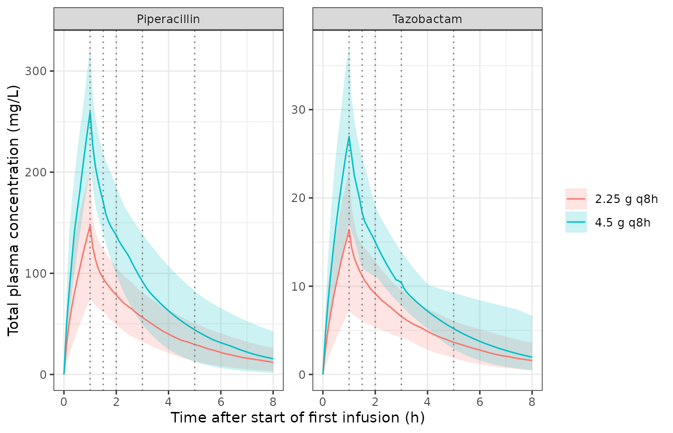
Simulated total plasma concentrations after the first dose (median and 5th-95th percentiles), with the paper’s sampling times (1, 1.5, 2, 3 and 5 h) marked. Compare with Figure 1 of Ishihara 2020 (observed concentration-time data).
Figure 4 – tazobactam probability of target attainment
The tazobactam PD target is an unbound AUC over 24 h of at least 96
ug h/mL (section 4.4), with 30% protein binding. At steady state the
24-h AUC equals the daily dose divided by clearance, so the target
reduces to CL <= 0.7 * D24 / 96. With a log-normal eta
on CL, the PTA has a closed form:
PTA = Phi( (log(0.7 * D24 / 96) - log(TVCL)) / omega_CL )
where TVCL = 5.00 + 0.0587 * (CLcr - 37.4) and
omega_CL^2 = 0.0715. Volumes and Q play no role, so this is
an exact read-out of the published clearance model. The points below
were digitised by the maintainers from Figure 4.
ini_taz <- ui_taz$theta
omega_taz <- ui_taz$omega
tvcl_taz <- function(crcl) exp(ini_taz[["lcl"]]) + ini_taz[["e_crcl_cl"]] * (crcl - 37.4)
pta_taz <- function(d24, crcl) {
  pnorm((log(0.7 * d24 / 96) - log(tvcl_taz(crcl))) / sqrt(omega_taz["etalcl", "etalcl"]))
}

# Digitised from Figure 4 (TAZ dose per administration, interval).
fig4 <- tibble::tribble(
  ~regimen,                ~d24, ~`10`, ~`20`, ~`30`, ~`40`, ~`50`, ~`60`,
  "TAZ 0.5 g q6h",         2000, 100,   100,   100,   100,   100,   100,
  "TAZ 0.5 g q8h",         1500, 100,   100,   100,   100,   100,   100,
  "TAZ 0.5 g q12h",        1000, 100,   99.5,  98,    94.8,  88.5,  78.5,
  "TAZ 0.25 g q6h",        1000, 100,   99,    98,    95.5,  89.5,  79,
  "TAZ 0.25 g q8h",         750, 97.5,  91,    83,    63.5,  44.5,  27,
  "TAZ 0.25 g q12h",        500, 67,    41,    20.5,  8,     2.5,   1
) |>
  pivot_longer(`10`:`60`, names_to = "CRCL", values_to = "pta_paper") |>
  mutate(CRCL = as.numeric(CRCL), pta_model = 100 * pta_taz(d24, CRCL),
         diff = pta_model - pta_paper)

ggplot(fig4, aes(CRCL, colour = regimen)) +
  geom_line(aes(y = pta_model)) +
  geom_point(aes(y = pta_paper)) +
  labs(x = "Creatinine clearance (mL/min)", y = "PTA of fAUC0-24 >= 96 (%)",
       colour = NULL, caption = "Lines: closed form from the packaged model; points: digitised Figure 4") +
  theme_bw()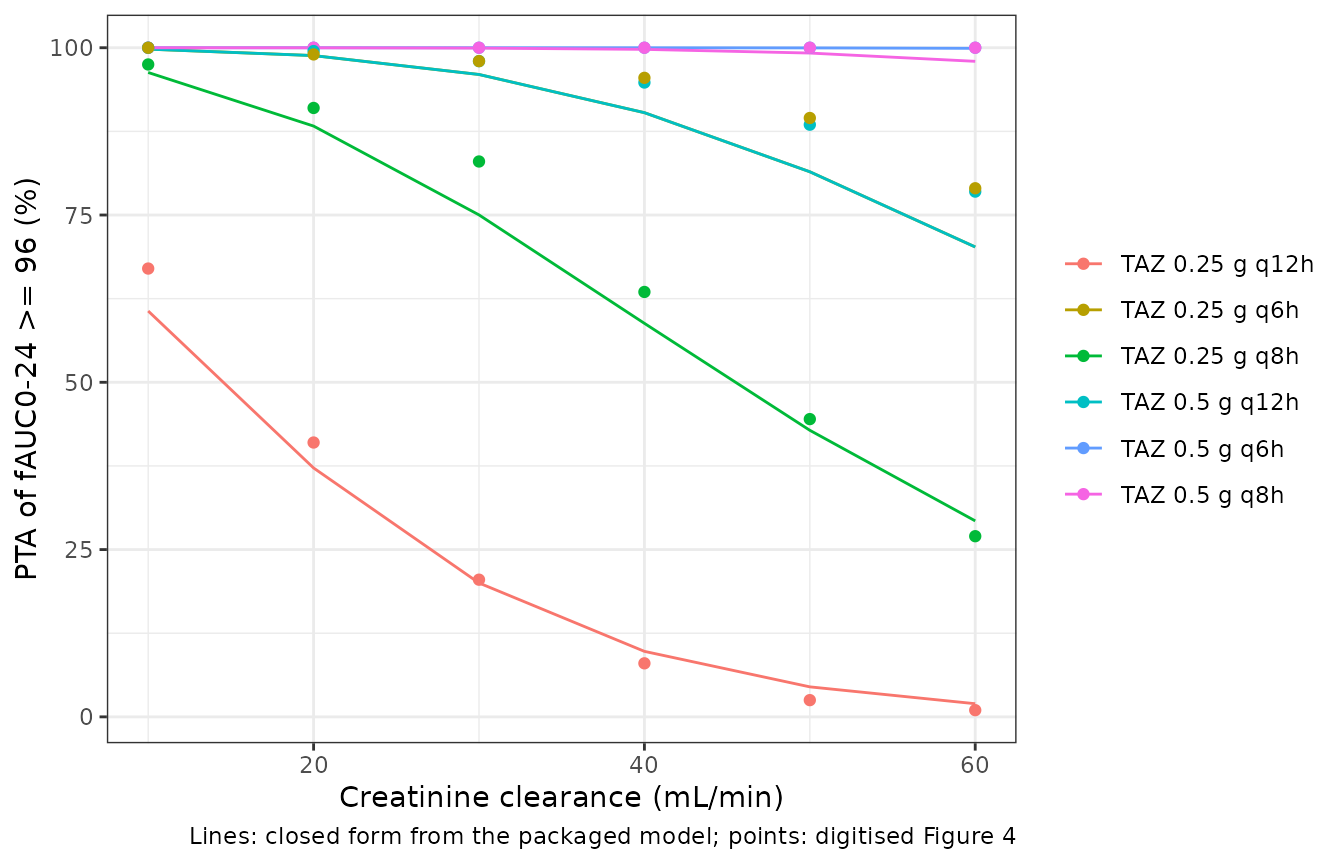
fig4 |>
  filter(d24 <= 1000) |>
  select(regimen, CRCL, pta_paper, pta_model, diff) |>
  mutate(across(c(pta_model, diff), \(x) round(x, 1))) |>
  rename(
    "Regimen" = regimen, "CLcr (mL/min)" = CRCL, "Figure 4 PTA (%)" = pta_paper,
    "Model PTA (%)" = pta_model, "Difference (pp)" = diff
  ) |>
knitr::kable()| Regimen | CLcr (mL/min) | Figure 4 PTA (%) | Model PTA (%) | Difference (pp) |
|---|---|---|---|---|
| TAZ 0.5 g q12h | 10 | 100.0 | 99.8 | -0.2 |
| TAZ 0.5 g q12h | 20 | 99.5 | 98.8 | -0.7 |
| TAZ 0.5 g q12h | 30 | 98.0 | 96.0 | -2.0 |
| TAZ 0.5 g q12h | 40 | 94.8 | 90.3 | -4.5 |
| TAZ 0.5 g q12h | 50 | 88.5 | 81.5 | -7.0 |
| TAZ 0.5 g q12h | 60 | 78.5 | 70.2 | -8.3 |
| TAZ 0.25 g q6h | 10 | 100.0 | 99.8 | -0.2 |
| TAZ 0.25 g q6h | 20 | 99.0 | 98.8 | -0.2 |
| TAZ 0.25 g q6h | 30 | 98.0 | 96.0 | -2.0 |
| TAZ 0.25 g q6h | 40 | 95.5 | 90.3 | -5.2 |
| TAZ 0.25 g q6h | 50 | 89.5 | 81.5 | -8.0 |
| TAZ 0.25 g q6h | 60 | 79.0 | 70.2 | -8.8 |
| TAZ 0.25 g q8h | 10 | 97.5 | 96.3 | -1.2 |
| TAZ 0.25 g q8h | 20 | 91.0 | 88.3 | -2.7 |
| TAZ 0.25 g q8h | 30 | 83.0 | 75.0 | -8.0 |
| TAZ 0.25 g q8h | 40 | 63.5 | 58.8 | -4.7 |
| TAZ 0.25 g q8h | 50 | 44.5 | 42.8 | -1.7 |
| TAZ 0.25 g q8h | 60 | 27.0 | 29.3 | 2.3 |
| TAZ 0.25 g q12h | 10 | 67.0 | 60.7 | -6.3 |
| TAZ 0.25 g q12h | 20 | 41.0 | 37.2 | -3.8 |
| TAZ 0.25 g q12h | 30 | 20.5 | 20.0 | -0.5 |
| TAZ 0.25 g q12h | 40 | 8.0 | 9.8 | 1.8 |
| TAZ 0.25 g q12h | 50 | 2.5 | 4.5 | 2.0 |
| TAZ 0.25 g q12h | 60 | 1.0 | 2.0 | 1.0 |
# Cross-check the closed form against a full ODE solve: steady-state 24-h AUC
# for a typical subject must equal D24 / TVCL.
typ <- rxode2::zeroRe(mod_taz)
#> ℹ parameter labels from comments will be replaced by 'label()'
ev_typ <- rxode2::et(amt = 250, rate = 250, ii = 8, addl = 2, ss = 1, cmt = "central") |>
  rxode2::et(seq(0, 24, by = 0.01), cmt = "central") |>
  as.data.frame() |>
  mutate(CRCL = 20)
s_typ <- rxode2::rxSolve(typ, ev_typ, addDosing = FALSE, returnType = "data.frame")
#> ℹ omega/sigma items treated as zero: 'etalcl', 'etalvc', 'etalq'
auc24 <- sum(diff(s_typ$time) * (head(s_typ$Cc, -1) + tail(s_typ$Cc, -1)) / 2)
# Deterministic: same parameters on both sides; only trapezoidal error remains.
stopifnot(abs(auc24 / (750 / tvcl_taz(20)) - 1) < 0.005)

# The regimens Figure 4 plots at 100% (0.5 g q6h / q8h; section 2.3: 'achieved
# PTA >= 90% in all patients') are 98.0-100% in the closed form; the lowest is
# 0.5 g q8h at CLcr 60. Deterministic, so a fixed bound is appropriate.
stopifnot(all(fig4$pta_model[fig4$d24 >= 1500] > 97))
# The regimens with a CLcr-dependent PTA: the published curves are digitised
# and the paper's PTA came from 1000 random subjects, so the gate is on the
# centre and a robust envelope of the paper-vs-model difference.
d_mid <- fig4$diff[fig4$d24 <= 1000]
stopifnot(abs(median(d_mid)) < 5, quantile(abs(d_mid), 0.9) < 12)
Table 4 and Figure 3 – piperacillin PK/PD breakpoints
The piperacillin PD target is an unbound concentration above the MIC for at least 50% of the dosing interval (50% fT > MIC) at steady state, with 30% protein binding and IIV but no residual error (section 4.4). Table 4 lists the highest MIC with PTA >= 90% for six regimens at six CLcr levels. The paper simulated 1000 subjects per scenario; here each scenario uses 200. The model’s breakpoints are systematically higher than Table 4; the Figure 1 check and the Assumptions and deviations section explain why the model, not Table 4, is taken as authoritative.
crcl_levels <- c(60, 50, 40, 30, 20, 10)
regimens <- tibble::tribble(
  ~regimen,      ~dose, ~ii,
  "4.5 g q6h",   4000,  6,
  "4.5 g q8h",   4000,  8,
  "4.5 g q12h",  4000, 12,
  "2.25 g q6h",  2000,  6,
  "2.25 g q8h",  2000,  8,
  "2.25 g q12h", 2000, 12
)
n_pta <- 200
scen <- tidyr::crossing(regimens, CRCL = crcl_levels) |>
  mutate(scenario = row_number())
subj <- scen |>
  tidyr::crossing(k = seq_len(n_pta)) |>
  mutate(id = row_number())

# Steady state via ss = 1, observed across one dosing interval.
ev_ss_dose <- subj |>
  mutate(time = 0, amt = dose, rate = dose, evid = 1, ss = 1, cmt = "central")
ev_ss_obs <- subj |>
  tidyr::crossing(time = seq(0, 12, by = 0.05)) |>
  filter(time <= ii) |>
  mutate(amt = 0, rate = 0, evid = 0, ss = 0, cmt = "central")
ev_ss <- bind_rows(ev_ss_dose, ev_ss_obs) |>
  select(id, time, amt, rate, ii, evid, ss, cmt, CRCL) |>
  arrange(id, time, desc(evid))
ev_ss$ii[ev_ss$evid == 0] <- 0

sim_ss <- rxode2::rxSolve(mod_pip, ev_ss, keep = "CRCL", returnType = "data.frame") |>
  left_join(select(subj, id, scenario), by = "id")

mics <- 2^(-4:7)
# Fraction of the interval with unbound concentration above each MIC; the last
# grid point (t = tau) duplicates t = 0 at steady state and is dropped.
ft <- sim_ss |>
  group_by(id, scenario) |>
  filter(time < max(time)) |>
  reframe(mic = mics, ft = vapply(mics, \(m) mean(0.7 * Cc > m), numeric(1)))
pta_pip <- ft |>
  group_by(scenario, mic) |>
  summarise(pta = mean(ft >= 0.5), .groups = "drop") |>
  left_join(scen, by = "scenario")
bp_model <- pta_pip |>
  group_by(regimen, CRCL) |>
  summarise(bp_model = max(c(0, mic[pta >= 0.9])), .groups = "drop")

table4 <- tibble::tribble(
  ~regimen,      ~`60`, ~`50`, ~`40`, ~`30`, ~`20`, ~`10`,
  "4.5 g q6h",   8,     16,    16,    32,    32,    64,
  "4.5 g q8h",   2,     4,     8,     8,     16,    32,
  "4.5 g q12h",  0.125, 0.25,  0.5,   1,     2,     4,
  "2.25 g q6h",  8,     8,     16,    16,    16,    32,
  "2.25 g q8h",  1,     2,     8,     8,     8,     16,
  "2.25 g q12h", 0.063, 0.125, 0.25,  0.5,   1,     2
) |>
  pivot_longer(-regimen, names_to = "CRCL", values_to = "bp_paper") |>
  mutate(CRCL = as.numeric(CRCL)) |>
  left_join(bp_model, by = c("regimen", "CRCL")) |>
  # The paper prints 0.0625 as 0.063.
  mutate(dilutions = round(log2(bp_model / ifelse(bp_paper == 0.063, 0.0625, bp_paper))))

table4 |>
  mutate(cell = paste0(bp_paper, " / ", bp_model)) |>
  select(regimen, CRCL, cell) |>
  pivot_wider(names_from = CRCL, values_from = cell) |>
  rename("Regimen (paper / model, ug/mL)" = regimen) |>
knitr::kable()| Regimen (paper / model, ug/mL) | 60 | 50 | 40 | 30 | 20 | 10 |
|---|---|---|---|---|---|---|
| 4.5 g q6h | 8 / 16 | 16 / 32 | 16 / 32 | 32 / 64 | 32 / 64 | 64 / 64 |
| 4.5 g q8h | 2 / 16 | 4 / 16 | 8 / 32 | 8 / 32 | 16 / 32 | 32 / 64 |
| 4.5 g q12h | 0.125 / 4 | 0.25 / 8 | 0.5 / 8 | 1 / 16 | 2 / 16 | 4 / 32 |
| 2.25 g q6h | 8 / 16 | 8 / 16 | 16 / 16 | 16 / 32 | 16 / 32 | 32 / 32 |
| 2.25 g q8h | 1 / 8 | 2 / 8 | 8 / 16 | 8 / 16 | 8 / 16 | 16 / 32 |
| 2.25 g q12h | 0.063 / 2 | 0.125 / 4 | 0.25 / 4 | 0.5 / 8 | 1 / 8 | 2 / 16 |
table(dilutions = table4$dilutions)
#> dilutions
#>  0  1  2  3  4  5
#>  3 15  4  6  4  4
# The packaged model does NOT reproduce Table 4: its breakpoints are higher in
# every cell, by one dilution for most q6h cells and by up to five for q12h
# (see "Table 4 is not reproducible" under Assumptions and deviations: Table 4
# is also inconsistent with the paper's own observed concentrations in
# Figure 1, which the model does reproduce -- gate below). The gate pins the
# direction and size of the disagreement so that a change in the model or the
# simulation that moves it is caught. A breakpoint is a step function of a
# 200-subject PTA near the 90% line, so a single cell can flip by one dilution
# between rxode2 builds; the gate is on the share of cells and the median.
stopifnot(
  mean(table4$dilutions >= 0) >= 0.9,
  median(table4$dilutions) >= 1,
  median(table4$dilutions) <= 4
)
Figure 1 – observed concentrations
Figure 1 plots the 100 observed concentrations of each drug against time after the start of an infusion, including pre-dose (time 0) samples taken during repeated dosing. The maintainers read the approximate range of each sampling time off the figure (log axes, so only to within about 10-20%). The simulated cohort’s 5th-95th percentiles at steady state should overlap these ranges, and its median should fall inside them.
fig1_ranges <- tibble::tribble(
  ~drug,          ~tad, ~obs_lo, ~obs_hi,
  "Piperacillin",    0,    5,     60,
  "Piperacillin",    1,  100,    450,
  "Piperacillin",    5,   17,    130,
  "Tazobactam",      0,    1,      8,
  "Tazobactam",      1,   10,     40,
  "Tazobactam",      5,    2,     15
)
t_last <- (n_dose - 1) * tau
fig1_sim <- sim |>
  mutate(tad = round(time - t_last, 1)) |>
  filter(tad %in% c(0, 1, 5)) |>
  group_by(drug, tad) |>
  summarise(
    sim_p05 = signif(quantile(Cc, 0.05), 3), sim_median = signif(median(Cc), 3),
    sim_p95 = signif(quantile(Cc, 0.95), 3), .groups = "drop"
  ) |>
  left_join(fig1_ranges, by = c("drug", "tad"))
fig1_sim |>
  rename(
    "Drug" = drug, "Time after start of infusion (h)" = tad,
    "Figure 1 low" = obs_lo, "Figure 1 high" = obs_hi,
    "Simulated 5th pct" = sim_p05, "Simulated median" = sim_median,
    "Simulated 95th pct" = sim_p95
  ) |>
knitr::kable()| Drug | Time after start of infusion (h) | Simulated 5th pct | Simulated median | Simulated 95th pct | Figure 1 low | Figure 1 high |
|---|---|---|---|---|---|---|
| Piperacillin | 0 | 2.070 | 13.30 | 44.80 | 5 | 60 |
| Piperacillin | 1 | 95.800 | 162.00 | 283.00 | 100 | 450 |
| Piperacillin | 5 | 12.700 | 35.30 | 82.20 | 17 | 130 |
| Tazobactam | 0 | 0.481 | 1.82 | 5.24 | 1 | 8 |
| Tazobactam | 1 | 10.200 | 18.80 | 30.50 | 10 | 40 |
| Tazobactam | 5 | 1.890 | 4.23 | 8.62 | 2 | 15 |
# Centre of the simulated cohort inside the observed range at every sampling
# time, for both drugs -- robust to which subjects land in the tails.
stopifnot(with(fig1_sim, all(sim_median > obs_lo & sim_median < obs_hi)))
pta_pip |>
  filter(mic %in% c(2, 4, 8, 16, 32, 64)) |>
  mutate(mic = factor(paste("MIC =", mic, "ug/mL"), levels = paste("MIC =", c(2, 4, 8, 16, 32, 64), "ug/mL"))) |>
  ggplot(aes(CRCL, 100 * pta, colour = regimen, shape = regimen)) +
  geom_line() +
  geom_point() +
  geom_hline(yintercept = 90, linetype = "dashed", colour = "grey50") +
  facet_wrap(~mic) +
  labs(x = "Creatinine clearance (mL/min)", y = "PTA of 50% fT > MIC (%)", colour = NULL, shape = NULL) +
  theme_bw()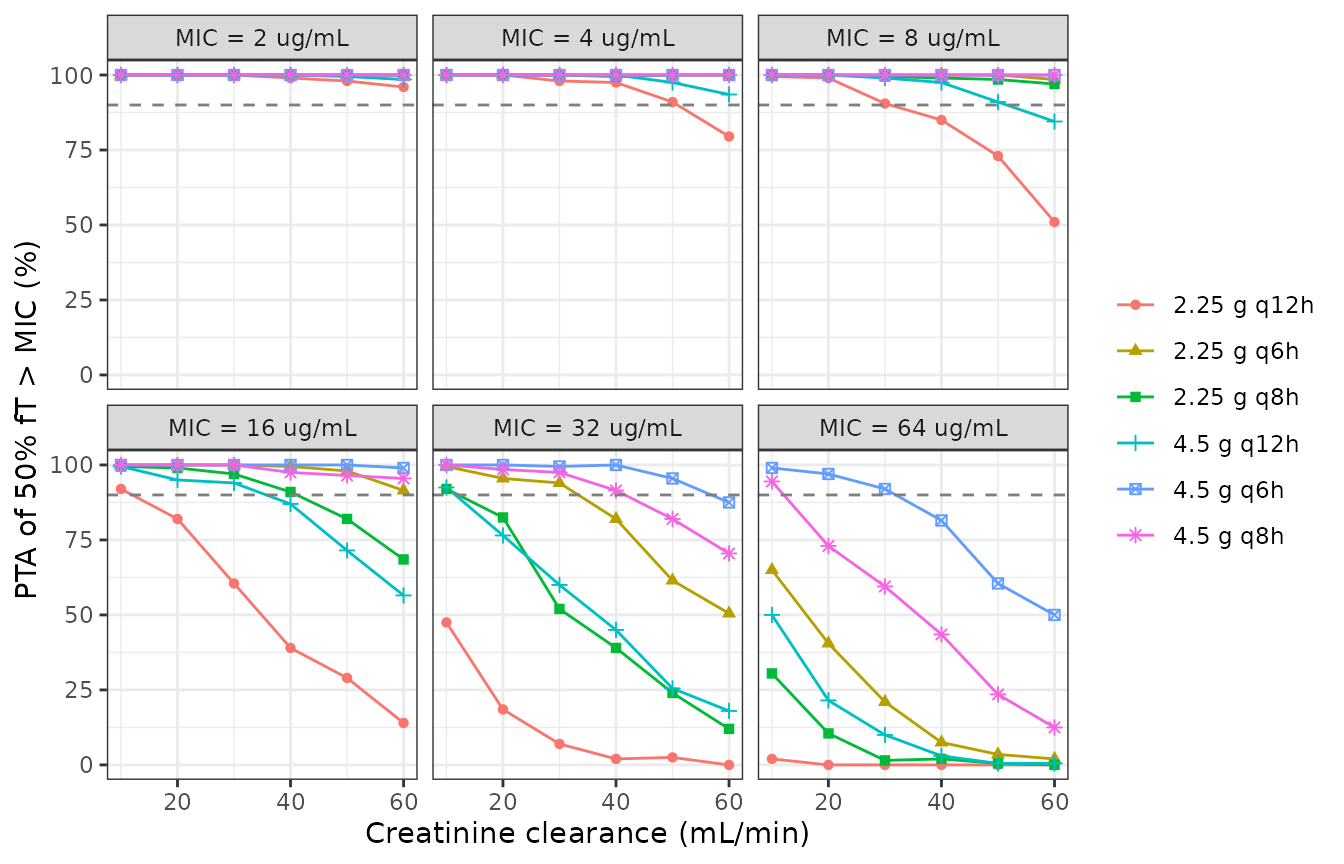
Model version of Figure 3 of Ishihara 2020: PTA of 50% fT > MIC for piperacillin by CLcr, one panel per MIC. The published panels are lower; see Assumptions and deviations.
PKNCA validation
conc <- sim |>
  filter(!is.na(Cc)) |>
  mutate(interval = ifelse(time <= tau, "first dose", "steady state")) |>
  select(id, time, Cc, drug, arm, interval)

dose_df <- bind_rows(
  mutate(ev_pip, drug = "Piperacillin"),
  mutate(ev_taz, drug = "Tazobactam")
) |>
  filter(evid == 1, time %in% c(0, (n_dose - 1) * tau)) |>
  mutate(interval = ifelse(time == 0, "first dose", "steady state")) |>
  select(id, time, amt, drug, arm, interval)

conc_obj <- PKNCA::PKNCAconc(conc, Cc ~ time | drug + arm + interval + id)
dose_obj <- PKNCA::PKNCAdose(dose_df, amt ~ time | drug + arm + interval + id)
intervals <- data.frame(
  start = c(0, (n_dose - 1) * tau),
  end = c(tau, n_dose * tau),
  interval = c("first dose", "steady state"),
  cmax = TRUE, tmax = TRUE, cmin = TRUE, auclast = TRUE
)
nca <- PKNCA::pk.nca(PKNCA::PKNCAdata(conc_obj, dose_obj, intervals = intervals))

nca$result |>
  filter(PPTESTCD %in% c("cmax", "cmin", "auclast")) |>
  group_by(drug, arm, interval, PPTESTCD) |>
  summarise(median = signif(median(PPORRES), 3), .groups = "drop") |>
  pivot_wider(names_from = PPTESTCD, values_from = median) |>
  rename(
    "Drug" = drug, "Arm" = arm, "Interval" = interval,
    "Cmax (mg/L)" = cmax, "Cmin (mg/L)" = cmin, "AUC0-8 (mg h/L)" = auclast
  ) |>
knitr::kable()| Drug | Arm | Interval | AUC0-8 (mg h/L) | Cmax (mg/L) | Cmin (mg/L) |
|---|---|---|---|---|---|
| Piperacillin | 2.25 g q8h | first dose | 396.0 | 147.0 | 0.00 |
| Piperacillin | 2.25 g q8h | steady state | 447.0 | 156.0 | 13.00 |
| Piperacillin | 4.5 g q8h | first dose | 668.0 | 260.0 | 0.00 |
| Piperacillin | 4.5 g q8h | steady state | 695.0 | 270.0 | 16.70 |
| Tazobactam | 2.25 g q8h | first dose | 45.8 | 16.4 | 0.00 |
| Tazobactam | 2.25 g q8h | steady state | 52.3 | 18.0 | 1.81 |
| Tazobactam | 4.5 g q8h | first dose | 73.0 | 27.0 | 0.00 |
| Tazobactam | 4.5 g q8h | steady state | 76.9 | 29.2 | 2.12 |
Comparison against published values
The paper reports no NCA. Its Discussion states the clearance of a
patient at the cohort mean CLcr (38.0 mL/min): 4.62 L/h for piperacillin
and 5.04 L/h for tazobactam. The steady-state AUC over one interval for
a typical patient at that CLcr must therefore equal dose / CL. The
simulated side is a typical-value (zeroRe()) solve at CLcr
= 38.0, not a cohort median, so both sides refer to the same reference
patient.
typ_subj <- data.frame(id = 1:2, CRCL = 38.0, dose_pip = c(2000, 4000), dose_taz = c(250, 500),
                       arm = c("2.25 g q8h", "4.5 g q8h"))
typ_sim <- bind_rows(
  rxode2::rxSolve(rxode2::zeroRe(mod_pip), make_events(typ_subj, "dose_pip"),
                  keep = "arm", returnType = "data.frame") |> mutate(drug = "Piperacillin"),
  rxode2::rxSolve(rxode2::zeroRe(mod_taz), make_events(typ_subj, "dose_taz"),
                  keep = "arm", returnType = "data.frame") |> mutate(drug = "Tazobactam")
) |>
  filter(time >= (n_dose - 1) * tau) |>
  mutate(group = paste(drug, arm))
#> ℹ parameter labels from comments will be replaced by 'label()'
#> ℹ omega/sigma items treated as zero: 'etalcl', 'etalvc', 'etalq'
#> Warning: multi-subject simulation without without 'omega'
#> ℹ parameter labels from comments will be replaced by 'label()'
#> ℹ omega/sigma items treated as zero: 'etalcl', 'etalvc', 'etalq'
#> Warning: multi-subject simulation without without 'omega'
typ_dose <- typ_sim |>
  distinct(group, id, drug, arm) |>
  mutate(time = (n_dose - 1) * tau,
         amt = ifelse(drug == "Piperacillin", typ_subj$dose_pip[id], typ_subj$dose_taz[id]))
typ_nca <- PKNCA::pk.nca(PKNCA::PKNCAdata(
  PKNCA::PKNCAconc(typ_sim, Cc ~ time | group + id),
  PKNCA::PKNCAdose(typ_dose, amt ~ time | group + id),
  intervals = data.frame(start = (n_dose - 1) * tau, end = n_dose * tau, auclast = TRUE)
))
reference <- typ_dose |>
  mutate(auclast = amt / ifelse(drug == "Piperacillin", 4.62, 5.04)) |>
  select(group, auclast)
cmp <- nlmixr2lib::ncaComparisonTable(
  typ_nca, reference, by = "group", units = c(auclast = "mg h/L")
)
knitr::kable(cmp)| NCA parameter | group | Reference | Simulated | % diff |
|---|---|---|---|---|
| AUClast (mg h/L) | Piperacillin 2.25 g q8h | 433 | 433 | +0.1% |
| AUClast (mg h/L) | Piperacillin 4.5 g q8h | 866 | 866 | +0.1% |
| AUClast (mg h/L) | Tazobactam 2.25 g q8h | 49.6 | 49.6 | +0.1% |
| AUClast (mg h/L) | Tazobactam 4.5 g q8h | 99.2 | 99.3 | +0.1% |
# Deterministic typical-value gate: the only differences are the rounding of
# the Discussion's 4.62 / 5.04 and trapezoidal error on a 0.1 h grid.
auc_chk <- typ_nca$result |>
  filter(PPTESTCD == "auclast") |>
  left_join(reference, by = "group")
stopifnot(all(abs(auc_chk$PPORRES / auc_chk$auclast - 1) < 0.01))
Assumptions and deviations
- Two independent models. The paper fitted piperacillin and tazobactam separately, so they are packaged as two files. When simulating the combination, their random effects are independent (no cross-drug correlation was estimated).
- Tazobactam CLcr term. No covariate reached significance for tazobactam (section 2.2.2); the authors retained the linear CLcr model with the smallest p-value by analogy with piperacillin. It is reproduced as published.
-
Additive-linear clearance with a proportional eta.
Section 4.3 states
theta_i = theta * exp(eta_i); the eta is applied to the whole covariate-adjusted CL, followingConil_2010_tobramycin. -
Variance scale. Tables 2 and 3 print omega^2 with
the matching log-normal CV (e.g. sqrt(exp(0.0705) - 1) = 27.0%), and
sigma^2 for residual error; the model stores the variances for omega and
the square roots for
propSd/addSd. The combined error uses separate epsilons (variances add), matchingCpred (1 + eps_prop) + eps_add. - Dose-reduction rule. The study reduced the dose when eGFR was below 50 mL/min; eGFR was not reported, so the virtual cohort uses Cockcroft-Gault CLcr for that split.
- CLcr levels outside the fitted range. The PTA scenarios at 10, 20 and 60 mL/min, taken from the paper, lie outside the observed CLcr range (21.5-59.1 mL/min); they extrapolate the linear clearance model exactly as the paper did.
- Figure 4 residuals. The model reproduces Figure 4’s ordering, the identical curves for the equal-daily-dose regimens (0.5 g q12h and 0.25 g q6h), and the 100% plateaus. The published curves are somewhat steeper in CLcr than the closed form (the paper is a few percentage points higher at low CLcr and lower at high CLcr). This cannot come from the structural model, since the closed form uses only the published CL equation and omega; it is most likely Monte Carlo noise in the paper’s 1000-subject simulation plus digitisation error. Parameters were not tuned.
- Table 4 and Figure 3 are not reproducible from Table 2. Simulated as described in section 4.4 (steady state, 1-h infusion, IIV only, 30% protein binding, 50% fT > MIC), the packaged piperacillin model gives PK/PD breakpoints above Table 4 in every cell: typically one dilution for the q6h regimens and three to five for q12h. The maintainers checked the alternative reading that the paper simulated a one-compartment model with V = Vc; that undershoots Table 4 by two to four dilutions, so it is not the explanation either. Table 4 also conflicts with the paper’s own data: Figure 1 shows pre-dose troughs of about 5-60 mg/L and 5-h concentrations of about 17-130 mg/L, mostly after 2-g doses. Unbound piperacillin at mid-interval is therefore far above the 0.063-4 ug/mL q12h breakpoints of Table 4. The model reproduces Figure 1 (gate above), and the tazobactam PTA of Figure 4, which depends only on CL and omega_CL, is reproduced with a median difference of about -2 percentage points (at most about 9). The discrepancy is therefore attributed to the paper’s piperacillin PTA simulation, not to the Table 2 estimates, which are packaged as published. Nothing was tuned. Figure 3 above is the model’s version and differs from the published panels in the same direction.
-
Unbound fraction. The 30% protein binding (fu =
0.7) used for the PK/PD analyses is applied in this vignette only; the
model’s
Ccis the total plasma concentration that was measured and fitted.