Flucloxacillin (Landersdorfer 2007)
Source:vignettes/articles/Landersdorfer_2007_flucloxacillin.Rmd
Landersdorfer_2007_flucloxacillin.RmdModel and source
- Citation: Landersdorfer CB, Kirkpatrick CMJ, Kinzig-Schippers M, Bulitta JB, Holzgrabe U, Drusano GL, Sorgel F. Population pharmacokinetics at two dose levels and pharmacodynamic profiling of flucloxacillin. Antimicrob Agents Chemother. 2007;51(9):3290-3297. doi:10.1128/AAC.01410-06
- Description: Three-compartment population PK model for IV flucloxacillin in healthy adult volunteers (Landersdorfer 2007) with linear renal and non-renal elimination. The structural model splits total clearance into a renal arm (CL_R = 5.37 L/h) and a non-renal arm (CL_NR = 2.73 L/h); their sum reproduces the derived total clearance CL_T = 8.10 L/h reported in Table 2. The renal arm also drives a cumulative urinary excretion compartment that the paper fits jointly with plasma. Distribution uses a shallow peripheral (V_2 = 2.61 L, CLic_shallow = 15.3 L/h) and a deep peripheral (V_3 = 2.17 L, CLic_deep = 1.23 L/h); central volume V_1 = 4.79 L. Between-subject variability is reported as a full 5x5 variance-covariance matrix (Table 3, natural-log scale) on CL_R, CL_NR, V_1, V_2, V_3; no BSV is included on the inter-compartmental clearances. Residual error is combined additive + proportional on both plasma concentrations (9.4% CV, 0.155 mg/L) and cumulative urinary amounts (20.9% CV, 1.04 mg). The 5-min infusion duration used in the study is supplied via dose records (DUR / RATE) rather than as a model parameter. No structural covariates were retained: the cohort was 10 healthy Caucasian adults (5 M / 5 F, weight 52-83 kg, age 23-34 years) and demographics are not used inside the model. Monte Carlo dose-attainment simulations in the paper (continuous, 4-h, 0.5-h infusions) reuse these PK parameters together with 96% protein binding.
- Article: https://doi.org/10.1128/AAC.01410-06
Population
Landersdorfer 2007 studied 10 healthy Caucasian adult volunteers (5 male, 5 female) in a randomised, two-way crossover trial at the Institute for Biomedical and Pharmaceutical Research (Nuernberg-Heroldsberg, Germany). The median body weight was 71 kg (range 52-83), median height 178 cm (range 165-190), and median age 25 years (range 23-34). All subjects had normal renal and hepatic function (Methods, Study participants; Results, Demographics).
Each subject received a single 500 mg dose and a single 1,000 mg dose of flucloxacillin as a 5-min intravenous infusion, separated by a >= 4-day washout period. Plasma and urine were sampled over 24 h post-infusion (Methods, Sampling schedule). The population PK fit pooled plasma and urine data across both dose levels using NONMEM V (FOCE-I, ADVAN 11 / TRANS 4 analytical solution); a three-compartment model with linear renal and non-renal elimination was selected over two-compartment and saturable-elimination alternatives based on a 200-point OFV improvement and visual predictive checks (Methods, Population PK analysis; Results, Population PK).
Source trace
The per-parameter origin is recorded as an in-file comment next to
each ini() entry in
inst/modeldb/specificDrugs/Landersdorfer_2007_flucloxacillin.R.
The table below collects them in one place.
| Equation / parameter | Value | Source location |
|---|---|---|
| Three-compartment ODE system (central + shallow peripheral + deep peripheral + cumulative urine) | n/a | Methods, Population PK analysis (equations for dX(1)/dt through dX(4)/dt) |
lcl_renal (renal CL CL_R) |
5.37 L/h | Table 2, CL_R |
lcl_nonren (non-renal CL CL_NR) |
2.73 L/h | Table 2, CL_NR |
lvc (central volume V_1) |
4.79 L | Table 2, V_1 |
lvp (shallow peripheral volume V_2) |
2.61 L | Table 2, V_2 |
lvp2 (deep peripheral volume V_3) |
2.17 L | Table 2, V_3 |
lq (central <-> shallow CLic_shallow) |
15.3 L/h | Table 2, CLic_shallow |
lq2 (central <-> deep CLic_deep) |
1.23 L/h | Table 2, CLic_deep |
| 5x5 BSV variance-covariance block on natural-log scale (CL_R, CL_NR, V_1, V_2, V_3) | see Table 3 entries | Table 3 (variance-covariance matrix) |
propSd (plasma proportional residual) |
0.094 (9.4% CV) | Table 2, CV_C |
addSd (plasma additive residual) |
0.155 mg/L | Table 2, SD_C |
propSd_urineAmt (urine proportional residual) |
0.209 (20.9% CV) | Table 2, CV_AU |
addSd_urineAmt (urine additive residual) |
1.04 mg | Table 2, SD_AU |
| 5-min infusion duration Tk_0 (fixed) | 5 min | Table 2, Tk_0 footnote (“not estimated”); supplied via dose record |
| No covariate effects retained | n/a | Methods, Individual PK model (only BSV variance-covariance is reported; no structural covariates discussed) |
Derived quantities (Table 2 footnotes b / c): total clearance CL_T = CL_R + CL_NR = 8.10 L/h; steady-state volume V_ss = V_1 + V_2 + V_3 = 9.57 L. These are not free parameters and are recovered automatically when the model is simulated.
Virtual cohort
The original observed concentration-time data are not redistributed with the nlmixr2lib package; the cohort below approximates the Landersdorfer 2007 trial demographics (n = 10 subjects per dose arm, both arms simulated to mirror the crossover design). The model has no structural covariates, so the cohort specification is just dosing.
set.seed(20070101L)

# Paper sampling schedule (Methods, Sampling schedule): pre-infusion (t=0),
# end of 5-min infusion, then 5, 10, 15, 20, 25, 45, 60, 75, 90 min and
# 2, 2.5, 3, 3.5, 4, 5, 6, 8, 24 h after end of infusion.
obs_times <- c(0,
               5/60,
               5/60 + c(5, 10, 15, 20, 25, 45, 60, 75, 90) / 60,
               5/60 + c(2, 2.5, 3, 3.5, 4, 5, 6, 8, 24))

make_cohort <- function(n, dose_mg, id_offset = 0L) {
  ids <- id_offset + seq_len(n)
  arm <- paste0(dose_mg, " mg")
  dosing <- tibble(
    id       = ids,
    time     = 0,
    amt      = as.numeric(dose_mg),
    evid     = 1L,
    cmt      = "central",
    dur      = 5 / 60,   # 5-min infusion (paper Tk_0)
    rate     = NA_real_,
    dose_arm = arm
  )
  obs <- tidyr::expand_grid(id = ids, time = obs_times) |>
    mutate(amt = NA_real_, evid = 0L, cmt = "Cc", dur = NA_real_,
           rate = NA_real_, dose_arm = arm)
  bind_rows(dosing, obs) |> arrange(id, time, desc(evid))
}

events <- bind_rows(
  make_cohort(n = 200L, dose_mg =  500, id_offset =    0L),
  make_cohort(n = 200L, dose_mg = 1000, id_offset = 1000L)
)

stopifnot(!anyDuplicated(unique(events[, c("id", "time", "evid")])))
Simulation
mod <- readModelDb("Landersdorfer_2007_flucloxacillin")
sim <- rxode2::rxSolve(mod, events = events, keep = "dose_arm") |>
  as.data.frame()
#> ℹ parameter labels from comments will be replaced by 'label()'
mod_typical <- rxode2::zeroRe(mod)
#> ℹ parameter labels from comments will be replaced by 'label()'
sim_typical <- rxode2::rxSolve(mod_typical, events = events, keep = "dose_arm") |>
  as.data.frame()
#> ℹ omega/sigma items treated as zero: 'etalcl_renal', 'etalcl_nonren', 'etalvc', 'etalvp', 'etalvp2'
#> Warning: multi-subject simulation without without 'omega'
Replicate published figures
# Replicates Figure 1 of Landersdorfer 2007: average plasma concentrations
# after 5-min IV infusions of 500 mg and 1,000 mg flucloxacillin. The paper's
# Figure 1 shows mean +/- SD profiles in linear and semi-log scales.
sim |>
  filter(time > 0, !is.na(Cc)) |>
  group_by(dose_arm, time) |>
  summarise(
    mean_Cc = mean(Cc),
    sd_Cc   = sd(Cc),
    .groups = "drop"
  ) |>
  ggplot(aes(time, mean_Cc, colour = dose_arm)) +
  geom_ribbon(aes(ymin = pmax(mean_Cc - sd_Cc, 1e-3),
                  ymax = mean_Cc + sd_Cc,
                  fill = dose_arm), alpha = 0.20, colour = NA) +
  geom_line() +
  scale_y_log10() +
  labs(x = "Time (h)", y = "Plasma flucloxacillin (mg/L, log scale)",
       colour = "Dose", fill = "Dose",
       title = "Figure 1 -- mean +/- SD plasma profiles after IV flucloxacillin",
       caption = "Replicates Landersdorfer 2007 Figure 1.")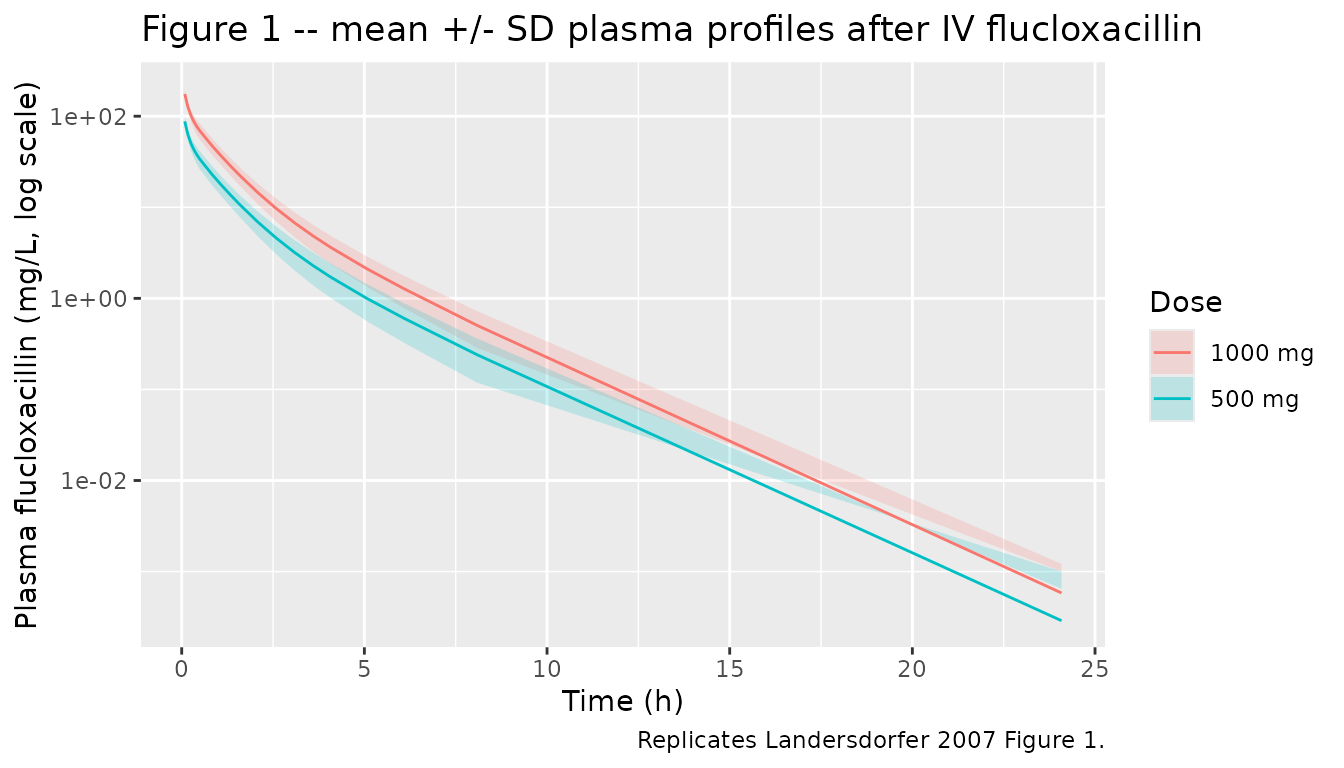
# Replicates Figure 2 of Landersdorfer 2007 (plasma VPC panel): median and
# prediction intervals over time, by dose group.
vpc_plasma <- sim |>
  filter(time > 0, !is.na(Cc)) |>
  group_by(dose_arm, time) |>
  summarise(
    Q10 = quantile(Cc, 0.10),
    Q25 = quantile(Cc, 0.25),
    Q50 = quantile(Cc, 0.50),
    Q75 = quantile(Cc, 0.75),
    Q90 = quantile(Cc, 0.90),
    .groups = "drop"
  )

ggplot(vpc_plasma, aes(time)) +
  geom_ribbon(aes(ymin = Q10, ymax = Q90, fill = dose_arm), alpha = 0.20) +
  geom_ribbon(aes(ymin = Q25, ymax = Q75, fill = dose_arm), alpha = 0.30) +
  geom_line(aes(y = Q50, colour = dose_arm)) +
  facet_wrap(~dose_arm, scales = "free_y") +
  scale_y_log10() +
  labs(x = "Time (h)", y = "Plasma flucloxacillin (mg/L, log scale)",
       colour = "Dose", fill = "Dose",
       title = "Figure 2 (plasma) -- VPC of simulated plasma concentrations",
       caption = "Replicates Landersdorfer 2007 Figure 2, plasma panel.")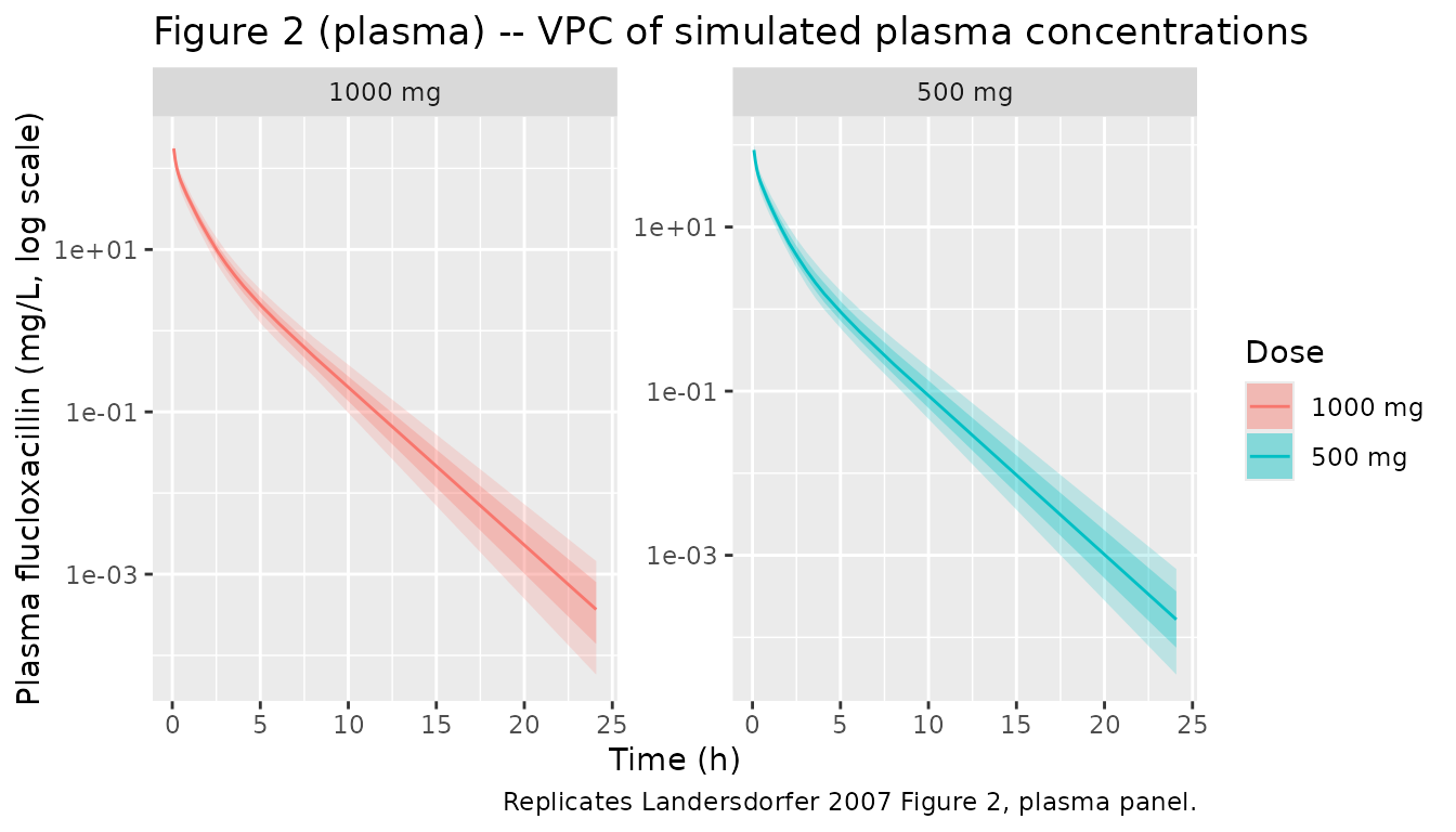
# Replicates Figure 2 of Landersdorfer 2007 (urine VPC panel): cumulative
# amount excreted unchanged in urine over 24 h.
vpc_urine <- sim |>
  filter(time > 0, !is.na(urineAmt)) |>
  group_by(dose_arm, time) |>
  summarise(
    Q10 = quantile(urineAmt, 0.10),
    Q25 = quantile(urineAmt, 0.25),
    Q50 = quantile(urineAmt, 0.50),
    Q75 = quantile(urineAmt, 0.75),
    Q90 = quantile(urineAmt, 0.90),
    .groups = "drop"
  )

ggplot(vpc_urine, aes(time)) +
  geom_ribbon(aes(ymin = Q10, ymax = Q90, fill = dose_arm), alpha = 0.20) +
  geom_ribbon(aes(ymin = Q25, ymax = Q75, fill = dose_arm), alpha = 0.30) +
  geom_line(aes(y = Q50, colour = dose_arm)) +
  facet_wrap(~dose_arm, scales = "free_y") +
  labs(x = "Time (h)", y = "Cumulative amount in urine (mg)",
       colour = "Dose", fill = "Dose",
       title = "Figure 2 (urine) -- VPC of simulated cumulative urinary amount",
       caption = "Replicates Landersdorfer 2007 Figure 2, urine panel.")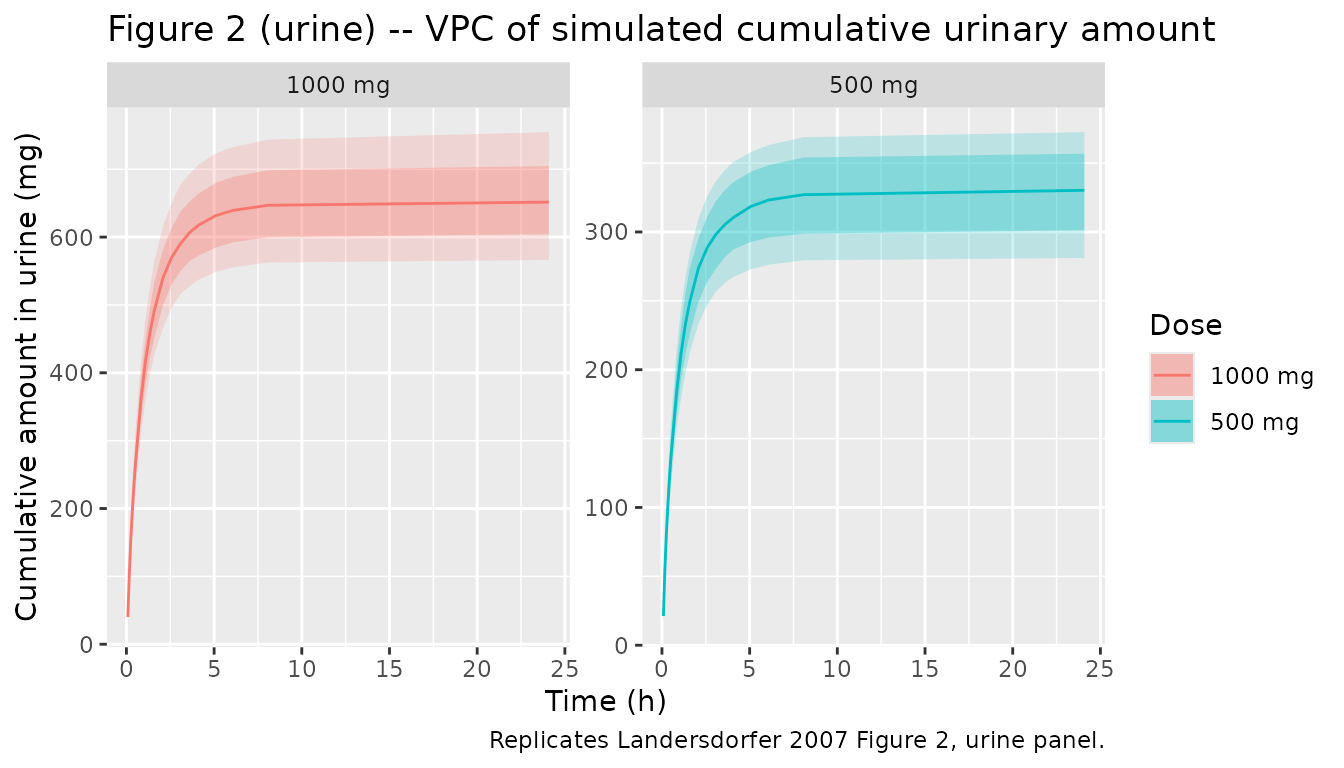
PKNCA validation
sim_nca <- sim |>
  filter(!is.na(Cc)) |>
  select(id, time, Cc, dose_arm)

dose_df <- events |>
  filter(evid == 1) |>
  select(id, time, amt, dose_arm)

conc_obj <- PKNCA::PKNCAconc(sim_nca, Cc ~ time | dose_arm + id,
                             concu = "mg/L", timeu = "h")
dose_obj <- PKNCA::PKNCAdose(dose_df, amt ~ time | dose_arm + id,
                             doseu = "mg")

intervals <- data.frame(
  start       = 0,
  end         = Inf,
  cmax        = TRUE,
  tmax        = TRUE,
  aucinf.obs  = TRUE,
  half.life   = TRUE,
  mrt.iv.obs  = TRUE
)

nca_res <- PKNCA::pk.nca(PKNCA::PKNCAdata(conc_obj, dose_obj, intervals = intervals))

nca_tbl <- as.data.frame(nca_res$result) |>
  filter(PPTESTCD %in% c("cmax", "tmax", "aucinf.obs", "half.life", "mrt.iv.obs")) |>
  group_by(dose_arm, PPTESTCD) |>
  summarise(
    geomean = exp(mean(log(pmax(PPORRES, 1e-9)), na.rm = TRUE)),
    cv_pct  = 100 * sqrt(exp(var(log(pmax(PPORRES, 1e-9)), na.rm = TRUE)) - 1),
    n_used  = sum(!is.na(PPORRES)),
    .groups = "drop"
  ) |>
  arrange(dose_arm, PPTESTCD)

knitr::kable(nca_tbl,
             digits   = 3,
caption = "Simulated NCA parameters (geometric mean, CV%) by dose arm.")| dose_arm | PPTESTCD | geomean | cv_pct | n_used |
|---|---|---|---|---|
| 1000 mg | aucinf.obs | 123.582 | 17.996 | 200 |
| 1000 mg | cmax | 174.013 | 13.818 | 200 |
| 1000 mg | half.life | 1.529 | 12.621 | 200 |
| 1000 mg | mrt.iv.obs | 1.235 | 13.050 | 200 |
| 1000 mg | tmax | 0.083 | 0.000 | 200 |
| 500 mg | aucinf.obs | 59.736 | 20.469 | 200 |
| 500 mg | cmax | 86.873 | 14.466 | 200 |
| 500 mg | half.life | 1.534 | 12.841 | 200 |
| 500 mg | mrt.iv.obs | 1.207 | 14.647 | 200 |
| 500 mg | tmax | 0.083 | 0.000 | 200 |
Comparison against published NCA (Table 1)
# Landersdorfer 2007 Table 1: noncompartmental analysis (geometric mean and CV%)
# from the n = 10 healthy-volunteer crossover trial. The 'mrt.iv.obs' label
# from PKNCA corresponds to the paper's "Mean residence time (h)" entry.
published <- tribble(
  ~dose_arm, ~param,        ~published_geomean, ~published_cv_pct,
  "500 mg",  "cmax",        86.8,               13,
  "500 mg",  "aucinf.obs",  500 / 8.16,         21,
  "500 mg",  "half.life",   1.40,               26,
  "500 mg",  "mrt.iv.obs",  1.18,               19,
  "1000 mg", "cmax",        167,                16,
  "1000 mg", "aucinf.obs",  1000 / 8.18,        20,
  "1000 mg", "half.life",   1.62,               25,
  "1000 mg", "mrt.iv.obs",  1.22,               14
) |>
  rename(PPTESTCD = param)

comparison <- published |>
  left_join(nca_tbl, by = c("dose_arm", "PPTESTCD")) |>
  mutate(pct_diff_geomean = 100 * (geomean - published_geomean) / published_geomean) |>
  select(dose_arm, PPTESTCD,
         published_geomean, published_cv_pct,
         simulated_geomean = geomean,
         simulated_cv_pct  = cv_pct,
         pct_diff_geomean,
         simulated_n_used  = n_used)

knitr::kable(comparison,
             digits = c(0, 0, 2, 1, 2, 1, 1, 0),
             caption = paste("Published (Landersdorfer 2007 Table 1) vs simulated",
                             "NCA parameters; AUCinf published values are derived",
                             "as dose / total-CL (CL_T = 8.16 L/h at 500 mg and",
                             "8.18 L/h at 1,000 mg per Table 1).",
                             "`simulated_n_used` is the number of simulated subjects",
                             "(of 200 per dose arm) for which PKNCA was able to",
                             "compute the parameter; the rest are excluded by",
                             "PKNCA's standard checks (e.g., too few terminal-phase",
"points)."))| dose_arm | PPTESTCD | published_geomean | published_cv_pct | simulated_geomean | simulated_cv_pct | pct_diff_geomean | simulated_n_used |
|---|---|---|---|---|---|---|---|
| 500 mg | cmax | 86.80 | 13 | 86.87 | 14.5 | 0.1 | 200 |
| 500 mg | aucinf.obs | 61.27 | 21 | 59.74 | 20.5 | -2.5 | 200 |
| 500 mg | half.life | 1.40 | 26 | 1.53 | 12.8 | 9.6 | 200 |
| 500 mg | mrt.iv.obs | 1.18 | 19 | 1.21 | 14.6 | 2.3 | 200 |
| 1000 mg | cmax | 167.00 | 16 | 174.01 | 13.8 | 4.2 | 200 |
| 1000 mg | aucinf.obs | 122.25 | 20 | 123.58 | 18.0 | 1.1 | 200 |
| 1000 mg | half.life | 1.62 | 25 | 1.53 | 12.6 | -5.6 | 200 |
| 1000 mg | mrt.iv.obs | 1.22 | 14 | 1.24 | 13.0 | 1.2 | 200 |
The paper’s noncompartmental analysis (Table 1) was performed on observed plasma samples from 10 subjects in a crossover design; the simulated NCA above uses 200 virtual subjects per dose arm and dense sampling, so the simulated CV% is expected to be somewhat tighter than the observed CV% (the observed CV% includes assay and within-subject variability that the typical-value simulation does not). Geometric means should agree closely (target <= 20% difference per the verification checklist). The half-life and MRT comparisons exercise the late-phase mixing among the three disposition compartments, which is the hardest part of the model to reproduce from a Table-2 / Table-3 read.
Assumptions and deviations
-
No structural covariates retained. The paper does
not include any covariate effects on PK parameters (Methods, Individual
PK model); the cohort was 10 healthy adults with normal renal and
hepatic function and the BSV model is a 5x5 variance-covariance block on
natural-log scale, not a covariate-driven structural model.
covariateDatais therefore empty. -
No BSV on inter-compartmental clearances. Table 2
footnote d explicitly records that BSV was not estimated for
CL_ic_shallow or CL_ic_deep “as estimation of these variance and
covariance terms did not significantly improve the objective function”
(Methods, Individual PK model). Reproduced as point-only
lqandlq2. -
5-min infusion duration is data-driven, not a model
parameter. The paper reports Tk_0 = 5 min as the structural
duration of the zero-order input but records it as a fixed protocol
constant (Table 2 footnote “not estimated”). In rxode2 / nlmixr2 the
infusion duration is supplied per dose record via
dur(orrate); the vignette cohort usesdur = 5/60 hto match the trial. Monte-Carlo dose-attainment simulations described in the paper (continuous, 4-h, 0.5-h infusions) reuse the same PK parameters and only change the dose record’s infusion duration. -
Variance reading. Table 3 reports the
variance-covariance matrix on the natural-log scale; the paper’s Methods
clarify that the “% CV” column in Table 2 is sqrt(omega^2) expressed as
a percentage rather than the back-transformed
log(1 + CV^2)form some popPK papers use. The Table 3 diagonals are therefore used directly asomega^2inini()rather than recomputed from the Table 2 CV%, which would introduce a rounding error. - AUCinf published reference is derived, not directly reported. Table 1 reports total clearance CL_T (8.16 L/h at 500 mg; 8.18 L/h at 1,000 mg) rather than AUCinf, so the comparison in the PKNCA section back-derives AUCinf = dose / CL_T. This is dimensionally equivalent and exact under the paper’s linear-PK conclusion (Results, Population PK; Discussion paragraph 6).
- Monte Carlo Simulation block omitted. The paper’s Figures 3 and 4 and Table 4 use the PK model to compute fT > MIC for various dosing regimens with 96% protein binding. Those simulations are dose-attainment analyses rather than PK validation, and are not reproduced here; the vignette is scoped to validating that the PK structural model + parameter set reproduce the paper’s primary PK observations (Figures 1-2 and Table 1).