Levonorgestrel implant release (Kim 2023)
Source:vignettes/articles/Kim_2023_levonorgestrel_implantRelease.Rmd
Kim_2023_levonorgestrel_implantRelease.RmdModel and source
Kim 2023 fitted ten candidate release functions to in vivo release data of the levonorgestrel (LNG) 150 mg two-rod subdermal implant (Jadelle) and carried two of them forward as the input function of a whole-body PBPK model. Both are packaged here as release-only models:
-
Kim_2023_levonorgestrel_firstOrderRelease: First-order in vivo release model for the levonorgestrel (LNG) 150 mg two-rod subdermal implant (Jadelle), fitted to explant residual-content data and Jadelle label release rates. Release-only: there is no levonorgestrel disposition. Only a fraction fdepot of the loaded dose is releasable (the paper’s Qmax = (1 - f) * Dose), and that releasable amount leaves the implant first-order at rate ka. The outputs are the cumulative amount released and the instantaneous release rate. Kim 2023 used this function as the input to a PK-Sim / MoBi whole-body PBPK model of levonorgestrel, which is not part of this model; the biexponential alternative the paper carried forward alongside it is Kim_2023_levonorgestrel_biexpRelease. -
Kim_2023_levonorgestrel_biexpRelease: Biexponential in vivo release model for the levonorgestrel (LNG) 150 mg two-rod subdermal implant (Jadelle), fitted to explant residual-content data and Jadelle label release rates. Release-only: there is no levonorgestrel disposition. The loaded dose is split between a fast pool (fraction frel, the paper’s Qb1 / Dose) released first-order at ka_fast and a slow pool (1 - frel) released first-order at ka_slow, so the whole load is eventually released. The implant is dosed twice at insertion, once into depot and once into depot2, each with the full load. The outputs are the cumulative amount released and the instantaneous release rate. Kim 2023 used this function as the input to a PK-Sim / MoBi whole-body PBPK model of levonorgestrel, which is not part of this model; the first-order alternative the paper carried forward alongside it is Kim_2023_levonorgestrel_firstOrderRelease. - Citation: Kim S, Cicali B, Pressly M, Da Silva L, Wendl T, Vozmediano V, Schmidt S, Cristofoletti R. Model-Based Analysis of In Vivo Release Data of Levonorgestrel Implants: Projecting Long-Term Systemic Exposure. Pharmaceutics. 2023;15(5):1393. doi:10.3390/pharmaceutics15051393. Parameter values from Table 2 (duplicated in Supplementary Table S1); release function from Table 1 (Weibull row, special case l = 1) and Equation (1).
- Article: https://doi.org/10.3390/pharmaceutics15051393
- Supplement (Table S1, Figure S1): https://www.mdpi.com/article/10.3390/pharmaceutics15051393/s1
The PBPK model the release functions feed (built in PK-Sim / MoBi,
from Cicali 2021, doi:10.1002/psp4.12572) is a platform model whose organ
volumes, flows and partition coefficients are not printed in either
paper, so it is not part of this package. The packaged models carry the
release step only; their outputs are the cumulative amount released from
the implant (released, mg) and the instantaneous release
rate (releaseRate, mg/day).
Population
The release functions were fitted to group-mean data, not to individual subjects (Section 2.2 and Figure 2):
- LNG content of explanted implants by time since insertion, from Callahan 2015 and Fuchs 2020 (two-rod implants removed for analysis up to 5 years after insertion; content measured by spectroscopy with HPLC confirmation). Released amount is the loaded 150 mg minus the measured residual content.
- The in vivo release rates of the Jadelle US product label – about 0.1 mg/day at month 1, 0.04 mg/day at 12 months and 0.03 mg/day from 24 months – converted to a released amount.
All subjects were healthy women using the implant for contraception.
The paper does not state how many explants contributed. The n = 321 in
its abstract is the Jadelle clinical-trial PK cohort used to check the
PBPK model (Figure 3), not the release fit. The same information is
available programmatically via
readModelDb("Kim_2023_levonorgestrel_firstOrderRelease")()$population.
Source trace
| Equation / parameter | Value | Source location |
|---|---|---|
First-order release,
Q(t) = Qmax * (1 - exp(-k1 * t))
|
n/a | Table 1, Weibull row, special case l = 1; Equation (1) |
Biexponential release,
Q(t) = Dose - Qb1 * exp(-kb1 * t) - (Dose - Qb1) * exp(-kb2 * t)
|
n/a | Table 1, Biexponential row |
Implant load Dose (both models) |
150 mg (fixed) | Table 2 |
lfdepot (first-order; Qmax / Dose) |
log(67.86 / 150) | Table 2 (Qmax = 67.86 mg); Section 3.1 (“45.3% of original LNG load”) |
lka (first-order; k1) |
log(0.0009) /day | Table 2 |
logitfrel (biexponential; Qb1 / Dose) |
logit(44.64 / 150) | Table 2 (Qb1 = 44.64 mg) |
lka_fast (biexponential; k1b) |
log(0.00127) /day | Table 2 |
lka_slow (biexponential; k2b) |
log(8.985e-5) /day | Table 2 |
| Residual error, inter-individual variability | none | Section 2.2 (unweighted nonlinear least squares; no variance reported) |
Table 2 and Supplementary Table S1 print identical values for both models.
Simulation
Each model is dosed with the 150 mg implant load at insertion (time
0). The biexponential model takes the load twice – once into
depot, once into depot2 – and splits it
between the two pools by bioavailability, so the two records together
release the full 150 mg once.
mod_fo <- rxode2::rxode2(readModelDb("Kim_2023_levonorgestrel_firstOrderRelease"))
mod_be <- rxode2::rxode2(readModelDb("Kim_2023_levonorgestrel_biexpRelease"))

days_per_month <- 365.25 / 12
obs_days <- seq(0, 60, by = 0.5) * days_per_month
load_mg <- 150

implant_events <- function(dose_cmts) {
  doses <- data.frame(id = 1L, time = 0, amt = load_mg, cmt = dose_cmts, evid = 1L)
  obs <- data.frame(id = 1L, time = obs_days, amt = 0, cmt = "released", evid = 0L)
  dplyr::bind_rows(doses, obs)
}

solve_release <- function(mod, dose_cmts, label) {
  sim <- rxode2::rxSolve(mod, events = implant_events(dose_cmts),
                         rtol = 1e-10, atol = 1e-12)
  as.data.frame(sim) |>
    dplyr::transmute(model = label, time, months = time / days_per_month,
                     released, releaseRate)
}

sim <- dplyr::bind_rows(
  solve_release(mod_fo, "depot", "First-order"),
  solve_release(mod_be, c("depot", "depot2"), "Biexponential")
)
Check against the published closed forms
The ODE solutions must reproduce the Table 1 release functions evaluated at the Table 2 estimates. Both sides use the same parameters, so the only difference is integration error.
closed_form <- function(model, t) {
  ifelse(
    model == "First-order",
    67.86 * (1 - exp(-0.0009 * t)),
    load_mg - 44.64 * exp(-0.00127 * t) - (load_mg - 44.64) * exp(-8.985e-5 * t)
  )
}
closed_rate <- function(model, t) {
  ifelse(
    model == "First-order",
    67.86 * 0.0009 * exp(-0.0009 * t),
    0.00127 * 44.64 * exp(-0.00127 * t) +
      8.985e-5 * (load_mg - 44.64) * exp(-8.985e-5 * t)
  )
}
chk <- sim |>
  dplyr::mutate(
    err_q = abs(released - closed_form(model, time)),
    err_rate = abs(releaseRate - closed_rate(model, time))
  )
chk |>
  dplyr::group_by(model) |>
  dplyr::summarise(max_abs_err_mg = max(err_q), max_abs_err_mg_per_day = max(err_rate))
#> # A tibble: 2 × 3
#>   model         max_abs_err_mg max_abs_err_mg_per_day
#>   <chr>                  <dbl>                  <dbl>
#> 1 Biexponential       2.73e-11               3.47e-14
#> 2 First-order         1.11e-11               1.00e-14
# Measured integration error is about 3e-11 mg at rtol = 1e-10; a transcription
# error in any parameter moves the 5-year released amount by whole milligrams.
stopifnot(max(chk$err_q) < 1e-5, max(chk$err_rate) < 1e-8)
Replicate Figure 2 (First-order and Biexponential panels)
label_rates <- data.frame(months = c(1, 12, 24), releaseRate = c(0.1, 0.04, 0.03))

sim_long <- sim |>
  tidyr::pivot_longer(c(released, releaseRate), names_to = "output", values_to = "value") |>
  dplyr::mutate(output = dplyr::recode(output,
    released = "LNG released (mg)",
    releaseRate = "LNG release rate (mg/day)"
  ))
label_long <- label_rates |>
  dplyr::rename(value = releaseRate) |>
  dplyr::mutate(output = "LNG release rate (mg/day)")

ggplot(sim_long, aes(months, value)) +
  geom_line() +
  geom_point(data = tidyr::crossing(label_long, model = unique(sim$model)),
             colour = "blue", size = 2) +
  facet_grid(output ~ model, scales = "free_y") +
  scale_x_continuous(breaks = seq(0, 60, by = 12)) +
  labs(x = "Months of use", y = NULL,
       caption = "Replicates the First-order and Biexponential panels of Figure 2 of Kim 2023 (typical curves; points: Jadelle label release rates).") +
  theme_bw()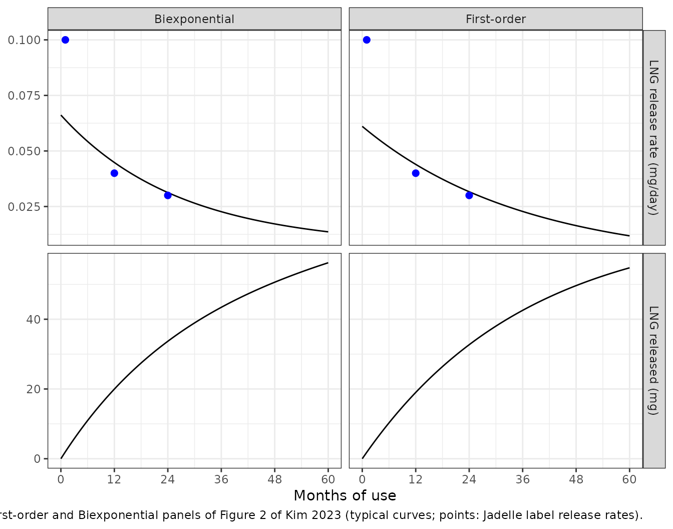
Both models start near 0.06 mg/day and fall to 0.03 mg/day by 24 months, matching the label’s 12- and 24-month rates; neither reaches the label’s 0.1 mg/day at month 1, as in the paper’s Figure 2. By 60 months both have released about 55-56 mg, the level of the last explant data point in Figure 2.
Published release landmarks
at_month <- function(m) sim |> dplyr::filter(abs(months - m) < 1e-8)
landmarks <- dplyr::bind_rows(
  at_month(1) |> dplyr::mutate(quantity = "Release rate at 1 month (mg/day)",
                               simulated = releaseRate, published = 0.1),
  at_month(12) |> dplyr::mutate(quantity = "Release rate at 12 months (mg/day)",
                                simulated = releaseRate, published = 0.04),
  at_month(24) |> dplyr::mutate(quantity = "Release rate at 24 months (mg/day)",
                                simulated = releaseRate, published = 0.03)
) |>
  dplyr::transmute(model, quantity, simulated = signif(simulated, 3), published,
                   pct_diff = round(100 * (simulated / published - 1), 1))
landmarks |>
  dplyr::rename(Model = model, Quantity = quantity, Simulated = simulated,
                `Jadelle label` = published, `% difference` = pct_diff) |>
knitr::kable()| Model | Quantity | Simulated | Jadelle label | % difference |
|---|---|---|---|---|
| First-order | Release rate at 1 month (mg/day) | 0.0594 | 0.10 | -40.6 |
| Biexponential | Release rate at 1 month (mg/day) | 0.0640 | 0.10 | -36.0 |
| First-order | Release rate at 12 months (mg/day) | 0.0440 | 0.04 | 10.0 |
| Biexponential | Release rate at 12 months (mg/day) | 0.0448 | 0.04 | 12.0 |
| First-order | Release rate at 24 months (mg/day) | 0.0316 | 0.03 | 5.3 |
| Biexponential | Release rate at 24 months (mg/day) | 0.0313 | 0.03 | 4.3 |
The 12- and 24-month rates are 4-12% above the label. The month-1 rate is 36-41% below the label for both models; the paper’s Figure 2 shows the same shortfall, since neither function reproduces the initial burst.
later <- dplyr::filter(landmarks, !grepl("1 month", quantity))
stopifnot(all(abs(later$pct_diff) < 15))
The first-order releasable fraction is
fdepot = 67.86 / 150 = 45.2% of the load, the paper’s
“45.3% of original LNG load”, close to the 50% non-releasable fraction
the authors assumed from ex vivo data at the end of a five-year trial
(Section 2.3).
Sino-implant (II) fits
To check the robustness of the approach, Kim 2023 refitted both
functions to the Sino-implant (II) explant data of Callahan 2015 and
reported the estimates in the text of Section 3.1 (to fewer significant
digits than Table 2): Qmax 75.6 mg and k1 0.0008 /day for the
first-order model; Qb1 14.95 mg, k1b 0.0062 /day and k2b 0.0002 /day for
the biexponential model. They are not packaged as separate models, but
they can be applied to the packaged models through
ini():
mod_fo_sino <- mod_fo |> rxode2::ini(lfdepot = log(75.6 / 150), lka = log(0.0008))
#> ℹ change initial estimate of `lfdepot` to `-0.685179010910768`
#> ℹ change initial estimate of `lka` to `-7.13089883029635`
mod_be_sino <- mod_be |>
  rxode2::ini(logitfrel = log((14.95 / 150) / (1 - 14.95 / 150)),
              lka_fast = log(0.0062), lka_slow = log(0.0002))
#> ℹ change initial estimate of `logitfrel` to `-2.20093378040193`
#> ℹ change initial estimate of `lka_fast` to `-5.08320598693109`
#> ℹ change initial estimate of `lka_slow` to `-8.51719319141624`

sim_sino <- dplyr::bind_rows(
  solve_release(mod_fo_sino, "depot", "First-order"),
  solve_release(mod_be_sino, c("depot", "depot2"), "Biexponential")
) |>
  dplyr::mutate(implant = "Sino-implant (II)")

dplyr::bind_rows(dplyr::mutate(sim, implant = "Jadelle"), sim_sino) |>
  ggplot(aes(months, released, colour = implant)) +
  geom_line() +
  facet_wrap(~model) +
  scale_x_continuous(breaks = seq(0, 60, by = 12)) +
  labs(x = "Months of use", y = "LNG released (mg)", colour = NULL,
       caption = "Jadelle (Table 2) versus Sino-implant (II) (Section 3.1) estimates.") +
  theme_bw()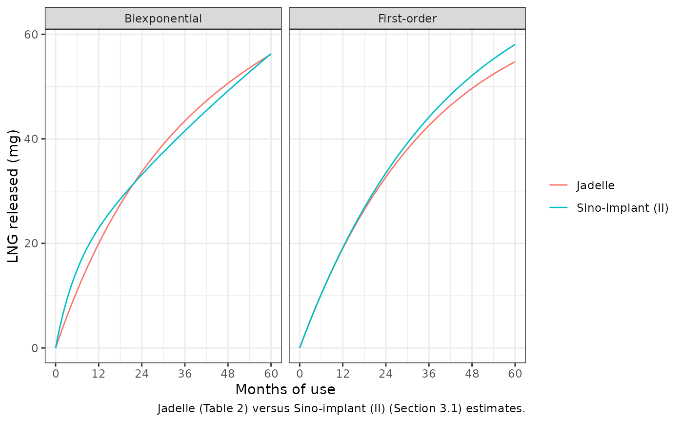
The paper interprets the Sino-implant biexponential fit as about 9.97% of the load released over roughly 5 months (1/0.0062 days) and the remaining 90.03% released slowly. The packaged parameterisation reproduces that split:
sino_theta <- mod_be_sino$theta
sino_split <- c(
  fast_pool_pct = 100 * rxode2::expit(sino_theta[["logitfrel"]]),
  fast_pool_mean_days = 1 / exp(sino_theta[["lka_fast"]])
)
sino_split
#>       fast_pool_pct fast_pool_mean_days
#>            9.966667          161.290323
# The paper's own figures: 9.97% of the load, over about 5 months (161 days).
stopifnot(abs(sino_split[["fast_pool_pct"]] - 9.97) < 0.01,
          abs(sino_split[["fast_pool_mean_days"]] - 161.3) < 0.1)
PKNCA
Not applicable. The packaged models describe release from the implant
only and produce no concentration, so there is nothing for
noncompartmental analysis to summarise. The release checks above
(closed-form identity and the published release-rate landmarks) are the
validation. To predict plasma levonorgestrel, couple
releaseRate to a levonorgestrel disposition model – for
example by replacing the released sink with that model’s
central compartment.
Assumptions and deviations
- Release-only. The paper’s systemic predictions (Figure 3) come from a PK-Sim / MoBi whole-body PBPK model whose structure is not printed, so they cannot be reproduced here and are not checked.
- No residual error or variability. The functions were fitted by unweighted nonlinear least squares to mean data (Section 2.2). Neither a residual variance nor any inter-individual variability was reported, so the models are deterministic. The 95% prediction bands of Figure 2 are not reproducible from the printed results.
-
Fractions instead of amounts. The paper estimates
QmaxandQb1in mg with the load fixed at 150 mg. They are stored as the fractionsfdepot = Qmax / 150andfrel = Qb1 / 150so the models are dose-driven. For a 150 mg implant the result is identical to the published functions (checked above). Using a different load assumes the releasable and fast-pool fractions scale with the load, which the paper did not test. -
Equation (1) versus Table 2. The PBPK input
function of Equation (1) is written with a non-releasable fraction
f“assumed to be 50%” (Section 2.3), while the fittedQmax = 67.86 mgimpliesf = 0.548; the paper notes thatQmaxis derived from(1 - f) * Dose. The packaged model uses the fitted Table 2 value. -
Equation (2) versus Table 1. Equation (2), the
biexponential PBPK input, multiplies the whole biexponential by
(1 - f), but the fitted function in Table 1 releases the full 150 mg (nof). Applying(1 - f) = 0.5would halve every release rate and contradict the release-rate panel of Figure 2, so the packaged model follows Tables 1 and 2. - Wide confidence intervals. All three biexponential estimates have 95% confidence intervals that span zero (Table 2); the paper chose the model for its biphasic mechanism rather than its precision (Section 4).
- Candidate models not packaged. Eight further release functions (Weibull, second-order, Korsmeyer-Peppas, Higuchi, zero-order, Hixson-Crowell, Peppas-Sahlin, Population Council) were fitted in the model-selection step and their estimates are in Supplementary Table S1. The paper did not carry them forward – the polynomial forms have no upper bound on the released amount, and the second-order fit has a negative adjusted R-squared – so they are not packaged.
- Month conversion. Figure axes in months are converted with 365.25 / 12 days per month.
- Errata. A EuropePMC search (2026-10-26) found no correction notice for this article.