Omeprazole intragastric pH (Soliman 2025)
Source:vignettes/articles/Soliman_2025_omeprazole.Rmd
Soliman_2025_omeprazole.RmdModel and source
- Citation: Soliman A, Rodriguez-Vera L, Alarcia-Lacalle A, et al. Leveraging Omeprazole PBPK/PD Modeling to Inform Drug-Drug Interactions and Specific Recommendations for Pediatric Labeling. Pharmaceutics. 2025;17(3):373. doi:10.3390/pharmaceutics17030373. PD model structure and the kdeg, kout, circadian and lag values from Liu D, Yang H, Jiang J, et al. Pharmacokinetic and Pharmacodynamic Modeling Analysis of Intravenous Esomeprazole in Healthy Volunteers. J Clin Pharmacol. 2016;56:816-826 (doi:10.1002/jcph.733); omeprazole kd from Katashima M, et al. Eur J Drug Metab Pharmacokinet. 1998;23:19-26 (doi:10.1007/BF03189822), both as tabulated in Soliman 2025 supplementary Table S1.
- Description: Semi-mechanistic intragastric-pH model for omeprazole in adults and children (Soliman 2025), the PD layer of the Soliman 2025 omeprazole PBPK/PD analysis. Plasma omeprazole irreversibly inactivates the gastric H+/K+-ATPase (relative activity E/E0, turnover kdeg, second-order inactivation kd * Cp acting after a 0.396 h lag); the active pump fraction scales a zero-order intragastric H+ secretion rate that carries a narrow night-time circadian dip, and H+ is cleared first-order (indirect-response model of Liu et al. 2016 for esomeprazole, with the omeprazole kd of Katashima et al. 1998). Meals dilute the gastric H+: each meal volume in mL is added to a dimensionless gastric-dilution state that relaxes back to 1 at the gastric-emptying rate kfe, and the observed H+ is the secreted H+ divided by that state; pH is capped at 7.4. Only this PD layer is reproduced here: the PK layer is a GastroPlus whole-body PBPK model whose organ volumes, blood flows, partition coefficients and enzyme abundances are platform database outputs the paper does not print, so the omeprazole plasma concentration is supplied by the user as the time-varying covariate CP_OMEPRAZOLE_NGML and meals are supplied as dose records into the gastric_volume compartment. The baseline H+ concentration defaults to the adult value; the paper’s pediatric baselines are listed in the population notes and are applied by overriding lrbase. No inter-individual variability or residual error is reported, so both are zero.
- Article: https://doi.org/10.3390/pharmaceutics17030373 (open access, PMC11944414)
- Supplement: https://www.mdpi.com/article/10.3390/pharmaceutics17030373/s1 (Table S1 lists the PD parameters; the section “Semi-mechanistic model to predict intragastric pH” gives Equations S1-S8)
Omeprazole is a proton-pump inhibitor: its acid-activated form binds the gastric H+/K+-ATPase covalently, so acid suppression outlasts the plasma exposure by days. Soliman 2025 built a GastroPlus whole-body PBPK model of omeprazole and its hydroxy and sulphone metabolites in adults, extrapolated it to children with CYP2C19 / CYP3A4 / CYP3A7 ontogeny, and linked the predicted plasma concentrations to a semi-mechanistic intragastric-pH model to compare acid suppression across ages, alone and under a hypothetical complete CYP3A inhibition.
Only the PD layer is packaged here. The PBPK layer
is a platform whole-body model: organ volumes and blood flows come from
the GastroPlus PEAR physiology module, tissue partition coefficients
from the Lukacova method, and enzyme abundances from the GastroPlus
database, none of which the paper tabulates, so the PK cannot be rebuilt
from the publication. The PD layer, by contrast, is printed in full in
the supplement and depends on the PK only through the plasma
concentration, which the user supplies as the time-varying covariate
CP_OMEPRAZOLE_NGML. Meals enter as dose records (in mL)
into the gastric_volume compartment.
The PD structure is the esomeprazole model of Liu et al. (2016): the
relative pump activity E/E0 turns over with rate
kdeg and is irreversibly inactivated at rate
kd * Cp; active pumps secrete H+ at a circadian zero-order
rate kin(t); H+ is cleared at kout; and meals
dilute the gastric contents. Soliman 2025 applied the model unchanged
across ages except for the fasting baseline H+ concentration and the
meal pattern.
Population
The PD model was not fitted to data in Soliman 2025; it was applied
to simulated reference populations of 4 months, 8 months, 2 years, 6
years and 37 years (100 subjects each, mean body weights 6.6, 9.11,
12.4, 23.5 and 85.27 kg; supplementary Table S6), dosed with omeprazole
20 mg once daily (adults) or 0.7 mg/kg once daily (children) for 8 days.
The PD parameters themselves come from healthy adult volunteers (Liu
2016 for esomeprazole, Katashima 1998 for the omeprazole
kd). The fasting baseline H+ falls with age from 0.79
mmol/L (pH 3.1) at 4 months to 40.1 mmol/L (pH 1.4) in adults (Table
S1). The PBPK layer behind the simulated concentrations was verified
against six published clinical PK studies (79 subjects, 0.3-45 years;
main Table 1).
Source trace
| Model element | Value | Source |
|---|---|---|
kdeg, H+/K+-ATPase turnover |
0.00827 1/h | Table S1; text below Eq. S8 (Liu 2016) |
kinact (paper kd), omeprazole
inactivation |
0.00388 1/h per ng/mL | Table S1; text below Eq. S8 (Katashima 1998) |
rbase (paper BASE), adult |
40.1 mmol/L (pH 1.4) | Table S1; supplementary text after Eq. S2 |
rbase, 6 y / 2 y / 8 mo / 4 mo |
31.62 / 16.59 / 1.2 / 0.79 mmol/L | Table S1 (applied below by overriding lrbase) |
kout |
3.83 1/h | Table S1; text after Eq. S2 |
amp_night (paper MA) |
537 | Table S1 (text says 398; see Assumptions) |
width_night (paper MW) |
0.0580 h | Table S1 (text says 1.25 h; see Assumptions) |
tpeak_night (paper MTmax) |
20.1 h | Table S1 (text says 22.4 h; see Assumptions) |
kfe, meal-dilution decay |
0.694 1/h | Table S1; text before Eq. S3 |
tlag, plasma-to-effect lag |
0.396 h | Table S1; text below Eq. S8 |
| Meal / milk volumes | see population$notes
|
Table S1 |
Circadian secretion kin(0), kin(t)
|
– | Eqs. S1, S2 |
| Meal-dilution state | – | Eqs. S3-S5 |
Pump activity E/E0
|
– | Eq. S6 |
| Secreted H+ | – | Eq. S7 |
Observed H+ H / VEf, pH cap 7.4 |
– | Eq. S8 and the paragraph above it |
Dimensional check of every ODE term (time in h):
| Equation | Term | Units |
|---|---|---|
d/dt(pump) |
kdeg, kdeg * pump
|
1/h (pump is unitless) |
kinact * pump * CP_OMEPRAZOLE_NGML |
(1/h per ng/mL) x ng/mL = 1/h | |
d/dt(hplus) |
kin * pump_lag |
mmol/L/h (kin0 = kout * rbase) |
kout * hplus |
1/h x mmol/L = mmol/L/h | |
d/dt(gastric_volume) |
meal input | mL/h added to a state whose fasting value is 1 |
kfe - kfe * gastric_volume |
1/h | |
| output | -log10(hplus / gastric_volume / 1000) |
pH (mmol/L converted to mol/L) |
The meal term adds millilitres to a dimensionless state. That is how the paper’s equations are written, and it is the reading that reproduces the paper’s Figure 5 (below); see Assumptions.
delay() needs the dense-output dop853
solver, so every solve below names it.
Mechanistic checks
Each of these compares a solve with a closed form that uses the same parameters, so the agreement is numerical and the tolerances are tight.
# 1. Drug-free, fasting: H+ starts at BASE and, because the circadian dip is
#    periodic and short, is back at BASE at every multiple of 24 h.
ev0 <- data.frame(
  id = 1, time = seq(0, 96, by = 0.1), evid = 0, amt = 0,
  cmt = "hplus", CP_OMEPRAZOLE_NGML = 0
)
s0 <- as.data.frame(rxSolve(ui, ev0, method = "dop853", returnType = "data.frame"))
h_day <- s0$hplus[s0$time %in% c(0, 24, 48, 72, 96)]
stopifnot(max(abs(h_day / rbase - 1)) < 1e-4)
c(fasting_pH = -log10(rbase / 1000), dip_max_pH = max(s0$gastric_ph))
#> fasting_pH dip_max_pH
#>   1.396856   2.109505

# 2. Constant plasma concentration: E/E0 follows
#    ss + (1 - ss) * exp(-(kdeg + kinact * C) * t), ss = kdeg / (kdeg + kinact * C)
#    (delayed by tlag in the pump_lag variable, not in the pump state).
cconst <- 2
ev1 <- data.frame(
  id = 1, time = seq(0, 600, by = 1), evid = 0, amt = 0,
  cmt = "pump", CP_OMEPRAZOLE_NGML = cconst
)
s1 <- as.data.frame(rxSolve(ui, ev1, method = "dop853", returnType = "data.frame"))
k_tot <- kdeg + kinact * cconst
ss <- kdeg / k_tot
pump_cf <- ss + (1 - ss) * exp(-k_tot * s1$time)
stopifnot(max(abs(s1$pump - pump_cf)) < 1e-6)

# 3. One 500 mL snack (bolus) at 2 h with no drug: the dilution state is
#    1 + 500 * exp(-kfe * (t - 2)) afterwards.
ev2 <- bind_rows(
  data.frame(id = 1, time = 2, evid = 1, amt = 500, cmt = "gastric_volume"),
  data.frame(id = 1, time = seq(0, 12, by = 0.25), evid = 0, amt = 0, cmt = "gastric_volume")
) |>
  arrange(time, desc(evid)) |>
  mutate(CP_OMEPRAZOLE_NGML = 0)
s2 <- as.data.frame(rxSolve(ui, ev2, method = "dop853", returnType = "data.frame"))
after <- s2$time >= 2
v_cf <- 1 + 500 * exp(-kfe * (s2$time[after] - 2))
stopifnot(max(abs(s2$gastric_volume[after] - v_cf) / v_cf) < 1e-6)

# 4. The pH output never exceeds the physiological cap of 7.4.
ev3 <- mutate(ev1, CP_OMEPRAZOLE_NGML = 5000)
s3 <- as.data.frame(rxSolve(ui, ev3, method = "dop853", returnType = "data.frame"))
stopifnot(max(s3$gastric_ph) <= 7.4)
Replicating Figure 5: day-8 intragastric pH by age
Figure 5 of Soliman 2025 shows, for each age group, the simulated median plasma omeprazole profile on day 8 (upper row) and the corresponding median intragastric pH (lower row). The maintainers digitised both median curves (omeprazole alone, without CYP3A inhibition) from the published figure. The digitised concentration is the model input here; the digitised pH is the comparison target. The concentration axis resolves about 17 ng/mL per pixel, so small tails are approximate.
# Day-8 median plasma omeprazole (ng/mL) at hours after the 168 h dose,
# digitised from Soliman 2025 Figure 5 (upper row, solid lines).
tc <- c(
  0, 0.25, 0.5, 0.75, 1, 1.25, 1.5, 1.75, 2, 2.25, 2.5, 2.75, 3, 3.25, 3.5,
  3.75, 4, 4.5, 5, 5.5, 6, 6.5, 7, 7.5, 8, 9:24
)
cp_dig <- list(
  adult = c(0, 52, 105, 152, 203, 225, 198, 176, 153, 124, 112, 94, 80, 67, 52, 48, 37, 33, 17, 17, 17, 17, 8, rep(0, 18)),
  `6y` = c(0, 203, 451, 543, 572, 542, 479, 415, 343, 285, 238, 197, 168, 137, 118, 98, 87, 64, 50, 33, 22, 17, 17, 17, rep(0, 17)),
  `2y` = c(0, 200, 454, 578, 610, 531, 453, 390, 333, 260, 217, 180, 153, 124, 109, 90, 73, 56, 33, 22, 17, 17, rep(0, 19)),
  `8mo` = c(0, 473, 829, 950, 945, 881, 793, 696, 590, 491, 417, 356, 293, 253, 212, 185, 162, 114, 83, 55, 47, 33, 18, 17, 17, rep(0, 16)),
  `4mo` = c(0, 427, 815, 1075, 1043, 946, 841, 733, 632, 532, 450, 383, 323, 270, 228, 188, 165, 122, 83, 55, 38, 32, 17, 17, rep(0, 17))
)

# Day-8 median intragastric pH at hours after the 168 h dose, digitised from
# Soliman 2025 Figure 5 (lower row, solid lines).
tp <- seq(0.5, 24, by = 0.5)
ph_dig <- list(
  adult = c(3.38, 3.85, 5.49, 5.45, 5.41, 5.38, 5.30, 5.15, 5.00, 5.30, 5.82, 5.68, 5.49, 5.31, 5.15, 5.04, 4.98, 4.78, 4.64, 4.45, 4.28, 4.96, 5.54, 5.37, 5.22, 5.07, 4.91, 4.73, 4.56, 4.39, 4.25, 4.09, 3.92, 3.77, 3.63, 3.47, 3.34, 3.22, 3.11, 3.23, 3.19, 2.82, 2.73, 2.68, 2.62, 2.59, 2.56, 2.54),
  `6y` = c(2.93, 3.86, 5.93, 6.13, 6.09, 6.04, 5.90, 5.69, 5.49, 5.62, 6.16, 5.97, 5.76, 5.58, 5.37, 5.23, 5.14, 4.95, 4.76, 4.58, 4.41, 4.97, 5.57, 5.41, 5.24, 5.06, 4.86, 4.71, 4.54, 4.36, 4.24, 4.07, 3.91, 3.76, 3.61, 3.49, 3.38, 3.25, 3.12, 3.18, 3.27, 2.91, 2.82, 2.76, 2.74, 2.71, 2.69, 2.69),
  `2y` = c(3.02, 3.86, 6.14, 6.14, 6.01, 5.86, 5.73, 5.54, 5.32, 5.47, 6.11, 5.93, 5.76, 5.58, 5.38, 5.23, 5.14, 4.97, 4.81, 4.63, 4.48, 4.78, 5.69, 5.53, 5.37, 5.21, 5.03, 4.86, 4.72, 4.53, 4.38, 4.22, 4.09, 3.93, 3.78, 3.66, 3.53, 3.42, 3.32, 3.43, 3.44, 3.14, 3.03, 2.99, 2.97, 2.93, 2.91, 2.88),
  `8mo` = c(4.52, 6.27, 7.86, 7.82, 7.65, 7.55, 7.35, 7.13, 6.88, 7.17, 7.54, 7.30, 7.09, 6.89, 6.69, 6.62, 6.46, 6.25, 6.06, 5.86, 5.71, 6.48, 7.16, 6.94, 6.78, 6.77, 6.85, 6.67, 6.49, 6.31, 6.17, 5.99, 5.81, 5.67, 5.49, 5.36, 5.18, 5.05, 4.92, 5.27, 4.86, 4.56, 4.46, 4.37, 4.29, 4.21, 4.17, 4.16),
  `4mo` = c(5.31, 5.83, 6.40, 6.27, 6.14, 6.00, 5.87, 5.71, 5.55, 5.84, 6.43, 6.27, 6.11, 5.97, 5.79, 5.63, 5.48, 5.93, 6.36, 6.18, 6.03, 5.87, 5.71, 5.58, 5.40, 5.75, 6.28, 6.09, 5.95, 5.79, 5.63, 5.50, 5.32, 5.84, 6.21, 6.07, 5.87, 5.74, 5.60, 5.82, 5.52, 5.75, 6.17, 5.95, 5.84, 5.66, 5.53, 5.40)
)
The age-specific inputs are the Table S1 baseline H+ and meal
pattern. Meals and milk feeds are 30-min infusions into
gastric_volume, snacks are boluses, and all times are hours
after each daily dose.
groups <- c("adult", "6y", "2y", "8mo", "4mo")
group_labels <- c(adult = "Adult", `6y` = "6 yr.", `2y` = "2 yr.", `8mo` = "8 mo.", `4mo` = "4 mo.")
base_mm <- c(adult = 40.1, `6y` = 31.62, `2y` = 16.59, `8mo` = 1.2, `4mo` = 0.79)

# One day's meals: time after dose (h), volume (mL), duration (h; 0 = bolus).
meals_for <- function(g) {
  vol <- switch(g,
    adult = c(540, 270, 600, 270, 630),
    `6y` = c(410, 180, 440, 180, 380),
    `2y` = c(290, 120, 360, 120, 330),
    `8mo` = c(330, 240, 330, 240, 510),
    NULL
  )
  if (g == "4mo") {
    return(data.frame(t = c(1, 5, 9, 13, 17, 21), vol = 120, dur = 0.5))
  }
  out <- data.frame(t = c(1, 3, 5, 8, 11), vol = vol, dur = c(0.5, 0, 0.5, 0, 0.5))
  if (g == "8mo") {
    out <- rbind(out, data.frame(t = 13, vol = 150, dur = 0.5))
  }
  out
}

make_events <- function(g, id) {
  day_meals <- meals_for(g)
  doses <- bind_rows(lapply(0:7, function(d) mutate(day_meals, t = t + 24 * d))) |>
    transmute(
      id = id, time = t, evid = 1, amt = vol, cmt = "gastric_volume",
      rate = ifelse(dur > 0, vol / dur, 0)
    )
  obs_t <- seq(0, 192, by = 0.05)
  # The day-8 concentration profile is repeated on every day (see Assumptions).
  cp_fun <- approxfun(tc, cp_dig[[g]], rule = 2)
  obs <- data.frame(
    id = id, time = obs_t, evid = 0, amt = 0, cmt = "gastric_volume", rate = 0
  )
  bind_rows(doses, obs) |>
    mutate(CP_OMEPRAZOLE_NGML = cp_fun(time %% 24)) |>
    arrange(time, desc(evid))
}

sim_fig5 <- bind_rows(lapply(seq_along(groups), function(i) {
  g <- groups[i]
  s <- as.data.frame(rxSolve(ui, make_events(g, i),
    params = c(lrbase = log(base_mm[[g]])), method = "dop853", returnType = "data.frame"
  ))
  s |>
    filter(time >= 168) |>
    transmute(group = g, tad = time - 168, gastric_ph, pump_lag, CP_OMEPRAZOLE_NGML)
}))
dig_df <- bind_rows(lapply(groups, function(g) data.frame(group = g, tad = tp, ph = ph_dig[[g]])))
lab <- function(x) factor(group_labels[x], levels = group_labels)
ggplot() +
  geom_line(data = sim_fig5, aes(tad + 168, gastric_ph, colour = "Model (this package)")) +
  geom_point(data = dig_df, aes(tad + 168, ph, colour = "Soliman 2025 Figure 5 (digitised median)"), size = 0.8) +
  geom_hline(yintercept = 4, linetype = "dotted", colour = "grey40") +
  geom_hline(yintercept = 6, linetype = "dashed", colour = "grey40") +
  facet_wrap(~ lab(group), nrow = 1) +
  scale_x_continuous(breaks = seq(168, 192, by = 6)) +
  labs(x = "Time (h)", y = "Intragastric pH", colour = NULL) +
  theme_bw() +
  theme(legend.position = "bottom")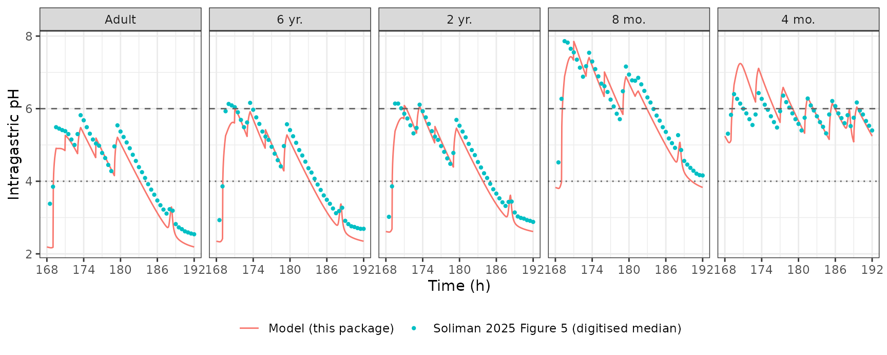
Replicates the lower row of Figure 5 of Soliman 2025 (omeprazole alone).
fig5_cmp <- dig_df |>
  group_by(group) |>
  mutate(model = approx(sim_fig5$tad[sim_fig5$group == group[1]],
    sim_fig5$gastric_ph[sim_fig5$group == group[1]],
    xout = tad
  )$y) |>
  summarise(
    `Median model - figure (pH)` = round(median(model - ph), 2),
    `Median absolute difference (pH)` = round(median(abs(model - ph)), 2),
    `90th percentile absolute difference (pH)` = round(quantile(abs(model - ph), 0.9), 2),
    .groups = "drop"
  ) |>
  mutate(group = lab(group)) |>
  arrange(group) |>
  rename(`Age group` = group)
knitr::kable(fig5_cmp)| Age group | Median model - figure (pH) | Median absolute difference (pH) | 90th percentile absolute difference (pH) |
|---|---|---|---|
| Adult | -0.35 | 0.35 | 0.54 |
| 6 yr. | -0.31 | 0.31 | 0.51 |
| 2 yr. | -0.26 | 0.27 | 0.33 |
| 8 mo. | -0.32 | 0.34 | 0.55 |
| 4 mo. | 0.04 | 0.18 | 0.82 |
# Structural gate: a wrong rate constant, baseline or meal volume moves the
# whole day-8 curve by a pH unit or more.
stopifnot(
  all(abs(fig5_cmp$`Median model - figure (pH)`) < 0.5),
  all(fig5_cmp$`90th percentile absolute difference (pH)` < 1.2)
)
The model tracks the published curves to within a few tenths of a pH unit in every age group: the morning rise when the dose and breakfast arrive, the saw-tooth from each meal, the narrow spike near 20 h after the dose that is the night-time secretion dip, and the decline back to the trough. The residual offset (the model runs slightly lower than the figure) is expected: the figure shows the median of 100 simulated subjects’ pH, whereas this solve feeds the median concentration through one typical subject, and pH is a non-linear function of concentration. In 8-month-old infants the published median reaches pH 7.9 on the morning peak, above the 7.4 cap the paper describes; the model applies the cap (see Assumptions).
Alternative readings of the supplement
The supplement gives two sets of circadian values (Table S1 and the text) and writes the meal volumes in mL. Re-running the adult panel under the alternatives shows why the packaged choices were made.
adult_dig <- data.frame(tad = tp, ph = ph_dig$adult)
score_adult <- function(params, meal_scale = 1) {
  ev <- make_events("adult", 1) |>
    mutate(amt = amt * meal_scale, rate = rate * meal_scale)
  s <- as.data.frame(rxSolve(ui, ev, params = params, method = "dop853", returnType = "data.frame")) |>
    filter(time >= 168)
  model <- approx(s$time - 168, s$gastric_ph, xout = adult_dig$tad)$y
  night <- adult_dig$tad >= 20.5
  c(
    `pH at the 168 h trough` = round(s$gastric_ph[1], 2),
    `Median model - figure, 20.5-24 h after dose (pH)` = round(median(model[night] - adult_dig$ph[night]), 2),
    `Median absolute difference, whole day (pH)` = round(median(abs(model - adult_dig$ph)), 2)
  )
}
alt <- rbind(
  `Table S1 circadian values, meals in mL (packaged)` = score_adult(c(lrbase = log(40.1))),
  `Supplement-text circadian values (MA 398, MW 1.25 h, MTmax 22.4 h)` = score_adult(c(
    lrbase = log(40.1), lamp_night = log(398), lwidth_night = log(1.25), ltpeak_night = log(22.4)
  )),
  `Meal volumes converted to litres` = score_adult(c(lrbase = log(40.1)), meal_scale = 1 / 1000)
)
knitr::kable(alt)| pH at the 168 h trough | Median model - figure, 20.5-24 h after dose (pH) | Median absolute difference, whole day (pH) | |
|---|---|---|---|
| Table S1 circadian values, meals in mL (packaged) | 2.19 | -0.34 | 0.35 |
| Supplement-text circadian values (MA 398, MW 1.25 h, MTmax 22.4 h) | 4.38 | 2.05 | 0.32 |
| Meal volumes converted to litres | 2.15 | -0.47 | 2.09 |
Figure 5 puts the adult trough at about pH 2.5 and shows a narrow spike near 20 h after the dose; only the Table S1 values give both. The text values switch acid secretion off for about two hours around 22.4 h, which holds the night-time pH near 4.5 where the figure has already fallen below 3; over the rest of the day the two sets agree, which is why the whole-day difference alone does not separate them. With the meals in litres the meal jumps shrink to a few hundredths of a pH unit and the saw-tooth of Figure 5 disappears.
Comparison with Figure 6: day-8 daily pH summaries
Figure 6 summarises day 8 as the average daily pH and the hours per day with pH above 4 and above 6 (median of 100 subjects; read off the published figure by the maintainers).
fig6 <- data.frame(
  group = groups,
  avg_pub = c(4.15, 4.32, 4.42, 6.00, 5.83),
  gt4_pub = c(15.3, 15.2, 15.7, 24, 24),
  gt6_pub = c(0, 2.5, 1.6, 13.8, 8.8)
)
dt <- 0.05
fig6_cmp <- sim_fig5 |>
  filter(tad < 24) |>
  group_by(group) |>
  summarise(
    avg_sim = mean(gastric_ph),
    gt4_sim = sum(gastric_ph > 4) * dt,
    gt6_sim = sum(gastric_ph > 6) * dt,
    .groups = "drop"
  ) |>
  left_join(fig6, by = "group") |>
  mutate(group = lab(group)) |>
  arrange(group)
fig6_cmp |>
  transmute(
    group,
    avg_sim = round(avg_sim, 2), avg_pub,
    gt4_sim = round(gt4_sim, 1), gt4_pub,
    gt6_sim = round(gt6_sim, 1), gt6_pub
  ) |>
  rename(
    `Age group` = group,
    `Average pH, model` = avg_sim, `Average pH, Figure 6` = avg_pub,
    `h pH > 4, model` = gt4_sim, `h pH > 4, Figure 6` = gt4_pub,
    `h pH > 6, model` = gt6_sim, `h pH > 6, Figure 6` = gt6_pub
  ) |>
knitr::kable()| Age group | Average pH, model | Average pH, Figure 6 | h pH > 4, model | h pH > 4, Figure 6 | h pH > 6, model | h pH > 6, Figure 6 |
|---|---|---|---|---|---|---|
| Adult | 4.00 | 4.15 | 14.1 | 15.3 | 0.0 | 0.0 |
| 6 yr. | 4.20 | 4.32 | 14.2 | 15.2 | 0.0 | 2.5 |
| 2 yr. | 4.38 | 4.42 | 14.8 | 15.7 | 0.7 | 1.6 |
| 8 mo. | 5.87 | 6.00 | 21.2 | 24.0 | 13.4 | 13.8 |
| 4 mo. | 6.02 | 5.83 | 24.0 | 24.0 | 10.9 | 8.8 |
The average daily pH and the hours above pH 4 follow the published ordering: older children and adults sit near pH 4 with roughly 15 h above pH 4, and infants under one year stay above pH 4 for the whole day. The hours above pH 6 are the most sensitive summary, because the day-8 curve of the older groups only grazes pH 6 at the post-meal peaks; there the model is a typical subject and the figure a population median.
In adults the paper cites a measured mean 24-h intragastric pH of 3.5 (SD 1.0) and 48.7 % (11.7 h) of the day above pH 4 after repeated 20 mg doses (Kirchheiner 2009) as agreeing with its simulations.
Assumptions and deviations
-
PD layer only. The GastroPlus PBPK layer is not
reproduced (platform physiology, partition coefficients and enzyme
abundances are not printed).
CP_OMEPRAZOLE_NGMLmust come from the user’s own omeprazole PK model or observed data. The simulations above use the day-8 median concentration curves digitised from Figure 5, repeated on days 1-7; the paper’s own PBPK profiles on the earlier days (which rise as omeprazole inhibits its own CYP2C19 metabolism) are not shown and could not be used. -
Circadian parameters: Table S1 values used.
Supplementary Table S1 lists
MA = 537,MW = 0.0580 h,MTmax = 20.1 h, while the supplementary text quotes 398, 1.25 h and 22.4 h (the values used by the same group in Pippa et al. 2024). Figure 5 shows a narrow spike about 20 h after each dose, which only the Table S1 values produce (a 1.25 h width gives a two-hour-wide plateau, and the text values put the adult trough at pH 4.4 instead of the published 2.5; see “Alternative readings” above). The Table S1 values are therefore taken as the ones the published simulations used. -
Meal units and the stomach-volume ratio. Equations
S3-S5 add meal volumes in mL to a state that relaxes back to 1, and
Equation S8 divides H+ by that state. Taken literally this is
dimensionally inconsistent, but it is the reading that reproduces the pH
jumps in Figure 5; converting the meals to litres (as the 1 L stomach
volume of Pippa et al. 2024 suggests) shrinks the meal jumps to a few
hundredths of a pH unit and leaves the adult curve about 2 pH units
below Figure 5 (see “Alternative readings”). Table S1 also lists an
age-specific stomach-volume ratio (
VEf= 1, 0.1036, 0.04866, 0.0375, 0.0352), but no printed equation uses it. In an exploratory solve by the maintainers, using it as the fasting value of the dilution state, or dividing the meal volumes by it, moved the 6-year, 2-year and 8-month curves further from Figure 5. It is therefore not part of the model. - Second snack volume. The text describes two snacks (3 h and 8 h after the dose) but Table S1 lists only one snack volume (“meal no. 2”); the 8 h snack is given the same volume. Figure 5 shows a small rise at 8 h in the adult and child panels.
-
4-month milk feeds. Equation S5 for 4-month-old
infants omits the
kfe - kfe * VEfemptying term of Equations S3-S4; without it the dilution would accumulate without limit, whereas Figure 5 shows a stable saw-tooth. The emptying term is kept for all ages. - pH cap. The 7.4 upper limit on pH stated in the supplement is applied, although the 8-month median in Figure 5 exceeds it on the morning peak.
-
Lag. The 0.396 h lag between plasma concentration
and effect is implemented by delaying the pump-activity state rather
than the concentration, which is equivalent because the pump equation
depends on time only through the concentration. The
pumpoutput is the undelayed state;pump_lagis the one that drives H+ secretion. -
Circadian clock.
Tin Equation S2 is taken as the time of day in hours after the once-daily dose, so model time 0 must be a dosing time. -
Pediatric baselines are applied by overriding
lrbase(above, throughrxSolve(params = )); the model file carries the adult value. - No variability. The paper reports no inter-individual variability or residual error for the PD model; its population spread came entirely from the PBPK layer. The additive pH error is fixed at zero.
- The CYP3A-inhibition (drug-drug interaction) arm is a PK change only; the same PD model applies to it with the user’s inhibited concentration profile.