Acetaminophen and metabolites (Mian 2019)
Source:vignettes/articles/Mian_2019_acetaminophen.Rmd
Mian_2019_acetaminophen.RmdModel and source
- Citation: Mian P, Valkenburg AJ, Allegaert K, Koch BCP, Breatnach CV, Knibbe CAJ, Tibboel D, Krekels EHJ (2019). Population pharmacokinetic modeling of acetaminophen and metabolites in children after cardiac surgery with cardiopulmonary bypass. J Clin Pharmacol 59(6):847-855. doi:10.1002/jcph.1373.
- Description: Parent-and-metabolites population PK model for intravenous acetaminophen (paracetamol) and its sulfate, glucuronide, and combined oxidative (cysteine + mercapturate) metabolites in infants and young children after cardiac surgery with cardiopulmonary bypass (Mian 2019). One-compartment plasma disposition for the parent and for each of the three metabolite pools. Formation clearance of each metabolite is a literature-assumed fixed fraction of the total acetaminophen elimination clearance (sulfation 0.49, glucuronidation 0.36, oxidation 0.10, unchanged 0.05). Total body weight enters the parent and all three metabolite elimination clearances as a linear (not allometric power) function centred on the population median weight of 6.1 kg. Down syndrome, age, sex, cardiopulmonary bypass time and RACHS-1 category were screened and none was retained.
- Article: https://doi.org/10.1002/jcph.1373 (open access; PMC6590134)
Mian and colleagues measured acetaminophen and three metabolite pools in scavenged blood samples from infants recovering from cardiac surgery with cardiopulmonary bypass, and fitted a parent-plus-metabolites population PK model in NONMEM 7.2. The structure (their Figure 1) is a one-compartment plasma model for the parent, feeding three one-compartment metabolite pools whose formation clearances are fixed fractions of the parent’s total elimination clearance.
Population
Thirty children contributed data: 17 with Down syndrome and 13 without (Table 1 of Mian 2019). Median age at surgery was 177 days (range 92-944) and median weight 6.1 kg (range 4.0-12.9). Thirteen of the 30 were male, so the cohort was 56.7% female. Surgery was for atrial septal defect, ventricular septal defect, atrioventricular septal defect or tetralogy of Fallot repair, with a median cardiopulmonary bypass time of about 110 minutes. Each child received three intravenous acetaminophen doses at 8-hour intervals, infused over 15 minutes, at 7.5 mg/kg (weight < 10 kg) or 15 mg/kg (weight >= 10 kg). The analysis used 161 acetaminophen, 161 sulfate, 161 glucuronide, 161 cysteine and 153 mercapturate concentrations; all acetaminophen glutathione samples were below the limit of quantification and that metabolite is absent from the model.
The same information is available programmatically via the model’s
population metadata
(readModelDb("Mian_2019_acetaminophen")()$population).
pop <- rxode2::rxode(readModelDb("Mian_2019_acetaminophen"))$population
#> ℹ parameter labels from comments will be replaced by 'label()'
tibble::tibble(Field = names(pop), Value = vapply(pop, function(x) paste(as.character(x), collapse = "; "), character(1))) |>
knitr::kable(caption = "Population metadata recorded with the model.")| Field | Value |
|---|---|
| species | human |
| n_subjects | 30 |
| n_studies | 1 |
| age_range | 92-944 days (inclusion criterion 3-36 months) |
| age_median | 177 days |
| weight_range | 4.0-12.9 kg |
| weight_median | 6.1 kg |
| sex_female_pct | 56.7 |
| race_ethnicity | NA |
| disease_state | Infants and young children in the immediate postoperative period after cardiac surgery with cardiopulmonary bypass for atrial septal defect, ventricular septal defect, atrioventricular septal defect or tetralogy of Fallot repair. 17 of 30 children had Down syndrome (trisomy 21). |
| dose_range | Three intravenous acetaminophen doses at 8-hour intervals, each infused over 15 minutes: 7.5 mg/kg for children < 10 kg and 15 mg/kg for children >= 10 kg. |
| regions | Ireland (Our Lady’s Children’s Hospital, Dublin) |
| n_observations | 161 acetaminophen, 161 acetaminophen sulfate, 161 acetaminophen glucuronide, 161 acetaminophen cysteine and 153 acetaminophen mercapturate concentrations (3-9 samples per patient). All acetaminophen glutathione concentrations were below the limit of quantification and that metabolite is not in the model. |
| notes | Demographics from Table 1 of Mian 2019. Acetaminophen concentrations were measured in scavenged blood samples from a previously published morphine / midazolam study in the same cohort. Sex is reported as 7/17 male in the Down-syndrome group and 6/13 male in the group without Down syndrome, i.e. 13/30 male and 17/30 (56.7%) female. Estimation used NONMEM 7.2 FOCE-I with ADVAN13. |
Source trace
Every ini() entry in
inst/modeldb/specificDrugs/Mian_2019_acetaminophen.R
carries an in-file comment naming its source location. They are
collected here for review.
| Equation / parameter | Value in the model | Source location |
|---|---|---|
lvc (V_APAP) |
7.96 L | Table 2, row V APAP (RSE 10%) |
lcl (CLE_APAP at 6.1 kg) |
1.50 - 0.54 = 0.96 L/h | Table 2, CLE APAP = theta1 * (BW/6.1) + theta2;
confirmed in the text as “0.96 L/h … for the typical child of 6.1
kg” |
e_wt_cl (theta1) |
1.50 L/h | Table 2, row theta 1 (RSE 27%) |
lvc_sulf |
0.68 L | Table 2, row V sulf (RSE 29%) |
lcle_sulf (at 6.1 kg) |
0.65 - 0.24 = 0.41 L/h | Table 2, CLE sulf = theta3 * (BW/6.1) + theta4
|
e_wt_cle_sulf (theta3) |
0.65 L/h | Table 2, row theta 3 (RSE 19%) |
lvc_gluc |
1.69 L | Table 2, row V gluc (RSE 29%) |
lcle_gluc (at 6.1 kg) |
1.41 - 0.53 = 0.88 L/h | Table 2, CLE gluc = theta5 * (BW/6.1) + theta6
|
e_wt_cle_gluc (theta5) |
1.41 L/h | Table 2, row theta 5 (RSE 21%) |
lvc_cysmer |
0.042 L | Table 2, row V ox (RSE 18%) |
lcle_cysmer (at 6.1 kg) |
40.86 - 1.26 = 39.60 L/h | Table 2, CLE ox = theta7 * (BW/6.1) + theta8
|
e_wt_cle_cysmer (theta7) |
40.86 L/h | Table 2, row theta 7 (RSE 25%) |
fm_sulf, fm_gluc, fm_cysmer,
fm_other
|
0.49, 0.36, 0.10, 0.05 | Methods, “Structural and Statistical Model” (assumed from the literature, not estimated) |
IIV etalvc … etalcle_cysmer
|
0.189, 0.185, 0.726, 0.189, 0.927, 0.129, 0.600, 0.552 | Table 2, block “Interindividual variability [omega^2]” |
Residual propSd*
|
sqrt of 0.146, 0.0507, 0.0813, 0.0494 | Table 2, block “Residual variability [sigma^2]” |
| One-compartment parent with four parallel elimination arms; one compartment per metabolite pool | n/a | Figure 1 and Results, “Structural and Statistical Model” |
| Linear (exponent fixed to 1) weight relationship on all four elimination clearances | n/a | Equation 1 and Results, “Covariate Model” |
The weight model, written two ways
Table 2 prints each elimination clearance as
CLE = theta_slope * (BW / 6.1) + theta_intercept. The model
file stores the algebraically identical centred form
CLE = CLE_6.1 + theta_slope * (BW / 6.1 - 1), CLE_6.1 = theta_slope + theta_interceptso that lcl / lcle_* hold the typical
clearance at the population median weight of 6.1 kg (the quantity the
paper quotes in its text) while e_wt_cl /
e_wt_cle_* hold theta_slope exactly as
printed. The chunk below checks the two forms agree to machine precision
over the studied weight range, which is the gate that protects the
rewrite.
mod <- readModelDb("Mian_2019_acetaminophen")
mod_typ <- rxode2::zeroRe(mod)
#> ℹ parameter labels from comments will be replaced by 'label()'

# Table 2, verbatim: slope and intercept for each of the four clearances.
tab2 <- tibble::tribble(
  ~analyte,   ~slope, ~intercept,
  "APAP",       1.50,      -0.54,
  "sulfate",    0.65,      -0.24,
  "glucuronide", 1.41,     -0.53,
  "oxidative",  40.86,     -1.26
)

wt_grid <- c(4.0, 5.0, 6.1, 8.0, 10.0, 12.9) # the studied 4.0-12.9 kg range

# One dose record per weight is enough to read the model's derived parameters
# back out of the solve. Observation rows use cmt = "Cc": this model declares
# four endpoints, so rxode2 assigns the observable slots AFTER the ODE states
# and cmt = "central" on an observation row is rejected. (lint_vignette.R's
# [cmt-observable] warning is a known false positive for declared
# multi-endpoint models.)
param_events <- tidyr::expand_grid(WT = wt_grid, time = c(0, 1)) |>
  dplyr::mutate(
    id = as.integer(factor(WT)),
    evid = ifelse(time == 0, 1L, 0L),
    amt = ifelse(time == 0, 7.5 * WT, NA_real_),
    rate = ifelse(time == 0, 7.5 * WT / 0.25, NA_real_),
    cmt = ifelse(time == 0, "central", "Cc")
  ) |>
  dplyr::arrange(id, time)

param_sim <- rxode2::rxSolve(
  mod_typ, param_events,
  omega = NA, useLinCmt = FALSE, maxsteps = 1e5, keep = "WT"
) |>
  as.data.frame() |>
  dplyr::distinct(WT, cl, cle_sulf, cle_gluc, cle_cysmer)
#> Warning: multi-subject simulation without without 'omega'

published <- tidyr::expand_grid(WT = wt_grid, tab2) |>
  dplyr::mutate(published = slope * (WT / 6.1) + intercept) |>
  dplyr::select(WT, analyte, published)

check_wt <- param_sim |>
  tidyr::pivot_longer(
    c(cl, cle_sulf, cle_gluc, cle_cysmer),
    names_to = "param", values_to = "modelled"
  ) |>
  dplyr::mutate(
    analyte = dplyr::recode(param,
      cl = "APAP", cle_sulf = "sulfate",
      cle_gluc = "glucuronide", cle_cysmer = "oxidative"
    )
  ) |>
  dplyr::left_join(published, by = c("WT", "analyte")) |>
  dplyr::mutate(abs_diff = abs(modelled - published))

# Deterministic identity between two algebraic forms of the same equation --
# not a cohort statistic -- so an exact tolerance is the right assertion.
stopifnot(
  nrow(check_wt) == length(wt_grid) * nrow(tab2),
  !anyNA(check_wt$published),
  max(check_wt$abs_diff) < 1e-10,
  # ...and every clearance stays positive across the studied weight range.
  all(check_wt$modelled > 0)
)

check_wt |>
  dplyr::select(WT, analyte, published, modelled) |>
  tidyr::pivot_wider(names_from = analyte, values_from = c(published, modelled)) |>
  dplyr::select(WT, published_APAP, modelled_APAP, published_sulfate, modelled_sulfate) |>
  dplyr::rename(
    "Weight (kg)" = WT,
    "CLE_APAP published (L/h)" = published_APAP,
    "CLE_APAP model (L/h)" = modelled_APAP,
    "CLE_sulf published (L/h)" = published_sulfate,
    "CLE_sulf model (L/h)" = modelled_sulfate
  ) |>
  knitr::kable(
    digits = 4,
    caption = "Table 2's printed clearance equations versus the packaged model, across the studied weight range. All four analytes agree to < 1e-10 L/h (only two shown for width)."
)| Weight (kg) | CLE_APAP published (L/h) | CLE_APAP model (L/h) | CLE_sulf published (L/h) | CLE_sulf model (L/h) |
|---|---|---|---|---|
| 4.0 | 0.4436 | 0.4436 | 0.1862 | 0.1862 |
| 5.0 | 0.6895 | 0.6895 | 0.2928 | 0.2928 |
| 6.1 | 0.9600 | 0.9600 | 0.4100 | 0.4100 |
| 8.0 | 1.4272 | 1.4272 | 0.6125 | 0.6125 |
| 10.0 | 1.9190 | 1.9190 | 0.8256 | 0.8256 |
| 12.9 | 2.6321 | 2.6321 | 1.1346 | 1.1346 |
Typical-value parameters at the median weight
typ <- param_sim |> dplyr::filter(WT == 6.1)
typ_vol <- rxode2::rxSolve(
  mod_typ, dplyr::filter(param_events, WT == 6.1),
  omega = NA, useLinCmt = FALSE, maxsteps = 1e5
) |>
  as.data.frame() |>
  dplyr::distinct(vc, vc_sulf, vc_gluc, vc_cysmer)

typical_cmp <- tibble::tribble(
  ~Quantity, ~Published, ~Modelled,
  "CLE_APAP at 6.1 kg (L/h)", 0.96, typ$cl,
  "V_APAP (L)", 7.96, typ_vol$vc,
  "CLE_sulf at 6.1 kg (L/h)", 0.65 - 0.24, typ$cle_sulf,
  "V_sulf (L)", 0.68, typ_vol$vc_sulf,
  "CLE_gluc at 6.1 kg (L/h)", 1.41 - 0.53, typ$cle_gluc,
  "V_gluc (L)", 1.69, typ_vol$vc_gluc,
  "CLE_ox at 6.1 kg (L/h)", 40.86 - 1.26, typ$cle_cysmer,
  "V_ox (L)", 0.042, typ_vol$vc_cysmer
) |>
  dplyr::mutate(`% diff` = 100 * (Modelled - Published) / Published)

# Deterministic: these are the ini() values read back through the solver.
stopifnot(max(abs(typical_cmp$`% diff`)) < 1e-8)

typical_cmp |>
knitr::kable(digits = c(0, 4, 4, 8), caption = "Typical-value parameters at the population median weight of 6.1 kg, against Table 2 of Mian 2019. The 0.96 L/h and 7.96 L values are quoted verbatim in the paper's Results.")| Quantity | Published | Modelled | % diff |
|---|---|---|---|
| CLE_APAP at 6.1 kg (L/h) | 0.960 | 0.960 | 0 |
| V_APAP (L) | 7.960 | 7.960 | 0 |
| CLE_sulf at 6.1 kg (L/h) | 0.410 | 0.410 | 0 |
| V_sulf (L) | 0.680 | 0.680 | 0 |
| CLE_gluc at 6.1 kg (L/h) | 0.880 | 0.880 | 0 |
| V_gluc (L) | 1.690 | 1.690 | 0 |
| CLE_ox at 6.1 kg (L/h) | 39.600 | 39.600 | 0 |
| V_ox (L) | 0.042 | 0.042 | 0 |
Virtual cohort
Original observed data are not publicly available. The cohort below matches the published weight range and the weight-banded dosing rule of the protocol. Weight is drawn uniformly over 4.0-12.9 kg, which spans the observed range; the paper reports only the median and range, not the shape of the distribution.
# set.seed() seeds R's RNG, not rxode2's simulation RNG, and rxode2's streams
# are partitioned per solver thread -- so this cohort is reproducible on one
# machine and different on a machine with a different thread count. Every
# assertion below is written to hold for any cohort the model can produce.
set.seed(20190601)
rxode2::rxSetSeed(20190601)

n_sub <- 120L

cohort <- tibble::tibble(
  id = seq_len(n_sub),
  WT = round(seq(4.0, 12.9, length.out = n_sub), 2)
) |>
  dplyr::mutate(
    # Postoperative pain protocol: 7.5 mg/kg below 10 kg, 15 mg/kg at or above.
    dose_mg = ifelse(WT < 10, 7.5 * WT, 15 * WT),
    treatment = ifelse(WT < 10, "7.5 mg/kg (< 10 kg)", "15 mg/kg (>= 10 kg)")
  )

# A log-spaced early grid resolves the 15-minute infusion peak and the fast
# oxidative-metabolite equilibration; a large IIV on the volumes otherwise
# costs several percent of AUC to trapezoidal error. The window stops at 36 h
# (> 6 typical parent half-lives). Carrying it further pushes the fastest
# subjects' oxidative pool into solver noise, where it goes slightly negative
# and PKNCA returns NA for lambda-z on those subjects.
obs_times <- sort(unique(c(
  0,
  exp(seq(log(0.01), log(1), length.out = 40)),
  seq(1.25, 12, by = 0.25),
  seq(12.5, 36, by = 0.5)
)))

doses_sd <- cohort |>
  dplyr::transmute(
    id, treatment, WT,
    time = 0, evid = 1L, amt = dose_mg,
    rate = dose_mg / 0.25, # 15-minute infusion
    cmt = "central"
  )

obs_sd <- tidyr::expand_grid(dplyr::select(cohort, id, treatment, WT), time = obs_times) |>
  dplyr::mutate(evid = 0L, amt = NA_real_, rate = NA_real_, cmt = "Cc")

events_sd <- dplyr::bind_rows(doses_sd, obs_sd) |>
  dplyr::arrange(id, time, dplyr::desc(evid))

stopifnot(!anyDuplicated(unique(events_sd[, c("id", "time", "evid")])))

# The three-dose regimen actually administered, for the profile figure.
doses_md <- tidyr::expand_grid(dplyr::select(cohort, id, treatment, WT, dose_mg), time = c(0, 8, 16)) |>
  dplyr::transmute(
    id, treatment, WT,
    time, evid = 1L, amt = dose_mg, rate = dose_mg / 0.25, cmt = "central"
  )

obs_md <- tidyr::expand_grid(
  dplyr::select(cohort, id, treatment, WT),
  time = sort(unique(c(seq(0, 32, by = 0.25), c(0, 8, 16) + 0.25)))
) |>
  dplyr::mutate(evid = 0L, amt = NA_real_, rate = NA_real_, cmt = "Cc")

events_md <- dplyr::bind_rows(doses_md, obs_md) |>
  dplyr::arrange(id, time, dplyr::desc(evid))
Simulation
# useLinCmt = FALSE: rxode2's automatic ODE-to-linCmt conversion corrupts the
# dvid -> cmt mapping for multi-output models.
# Tight tolerances: the oxidative pool's elimination rate constant is of the
# order of 1000 /h, which is stiff relative to the parent's 0.12 /h, and the
# default absolute tolerance leaves visible noise on its far tail.
sim_sd <- rxode2::rxSolve(
  mod, events_sd,
  keep = c("treatment", "WT"), useLinCmt = FALSE,
  maxsteps = 1e5, atol = 1e-12, rtol = 1e-10
) |>
  as.data.frame()
#> ℹ parameter labels from comments will be replaced by 'label()'

sim_md <- rxode2::rxSolve(
  mod, events_md,
  keep = c("treatment", "WT"), useLinCmt = FALSE, maxsteps = 1e5
) |>
  as.data.frame()

# Guard against the silent zeroRe failure mode: a typical-value solve must
# return a single clearance per weight.
stopifnot(dplyr::n_distinct(round(dplyr::filter(param_sim, WT == 6.1)$cl, 10)) == 1L)

# The model must not have been auto-solved analytically: all four ODE states
# have to survive into the output, or the metabolite arms would be silently
# discarded.
stopifnot(
  is.null(rxode2::rxode(mod)$linCmt),
  all(c("central", "central_sulf", "central_gluc", "central_cysmer") %in% rxode2::rxode(mod)$state),
  all(c("Cc", "Cc_sulf", "Cc_gluc", "Cc_cysmer") %in% names(sim_sd))
)
#> ℹ parameter labels from comments will be replaced by 'label()'
#> ℹ parameter labels from comments will be replaced by 'label()'

# No analyte may decay into negative solver noise inside the NCA window --
# PKNCA would take log() of a negative value and silently return NA for
# lambda-z and AUC0-inf on those subjects.
stopifnot(
  min(sim_sd$Cc, na.rm = TRUE) >= 0,
  min(sim_sd$Cc_sulf, na.rm = TRUE) >= 0,
  min(sim_sd$Cc_gluc, na.rm = TRUE) >= 0,
  min(sim_sd$Cc_cysmer, na.rm = TRUE) >= 0
)
Replicate published figures
Figure 3 – typical acetaminophen profile after a single 7.5 mg/kg dose
Figure 3 of Mian 2019 shows the population-predicted acetaminophen concentration in a typical 6.1-kg child after a single 7.5 mg/kg intravenous dose infused over 15 minutes. Only the cardiac-surgery arm is reproducible from this paper; see Assumptions and deviations for why the non-cardiac (Prins) comparator is not.
typ_events <- dplyr::bind_rows(
  tibble::tibble(
    id = 1L, WT = 6.1, time = 0, evid = 1L,
    amt = 7.5 * 6.1, rate = 7.5 * 6.1 / 0.25, cmt = "central"
  ),
  tibble::tibble(
    id = 1L, WT = 6.1,
    time = sort(unique(c(exp(seq(log(1e-3), log(1), length.out = 60)), seq(1, 24, by = 0.05)))),
    evid = 0L, amt = NA_real_, rate = NA_real_, cmt = "Cc"
  )
) |>
  dplyr::arrange(time, dplyr::desc(evid))

sim_typ <- rxode2::rxSolve(
  mod_typ, typ_events,
  omega = NA, useLinCmt = FALSE, maxsteps = 1e5, atol = 1e-12, rtol = 1e-10
) |>
  as.data.frame()

obs_typ <- dplyr::filter(sim_typ, time > 0)

sim_typ |>
  dplyr::filter(time > 0) |>
  ggplot(aes(time, Cc)) +
  geom_line(linewidth = 0.9) +
  labs(
    x = "Time (h)", y = "Acetaminophen (mg/L)",
    title = "Typical 6.1 kg child, single 7.5 mg/kg IV over 15 min",
    caption = "Replicates the cardiac-surgery arm (solid line) of Figure 3 of Mian 2019."
  )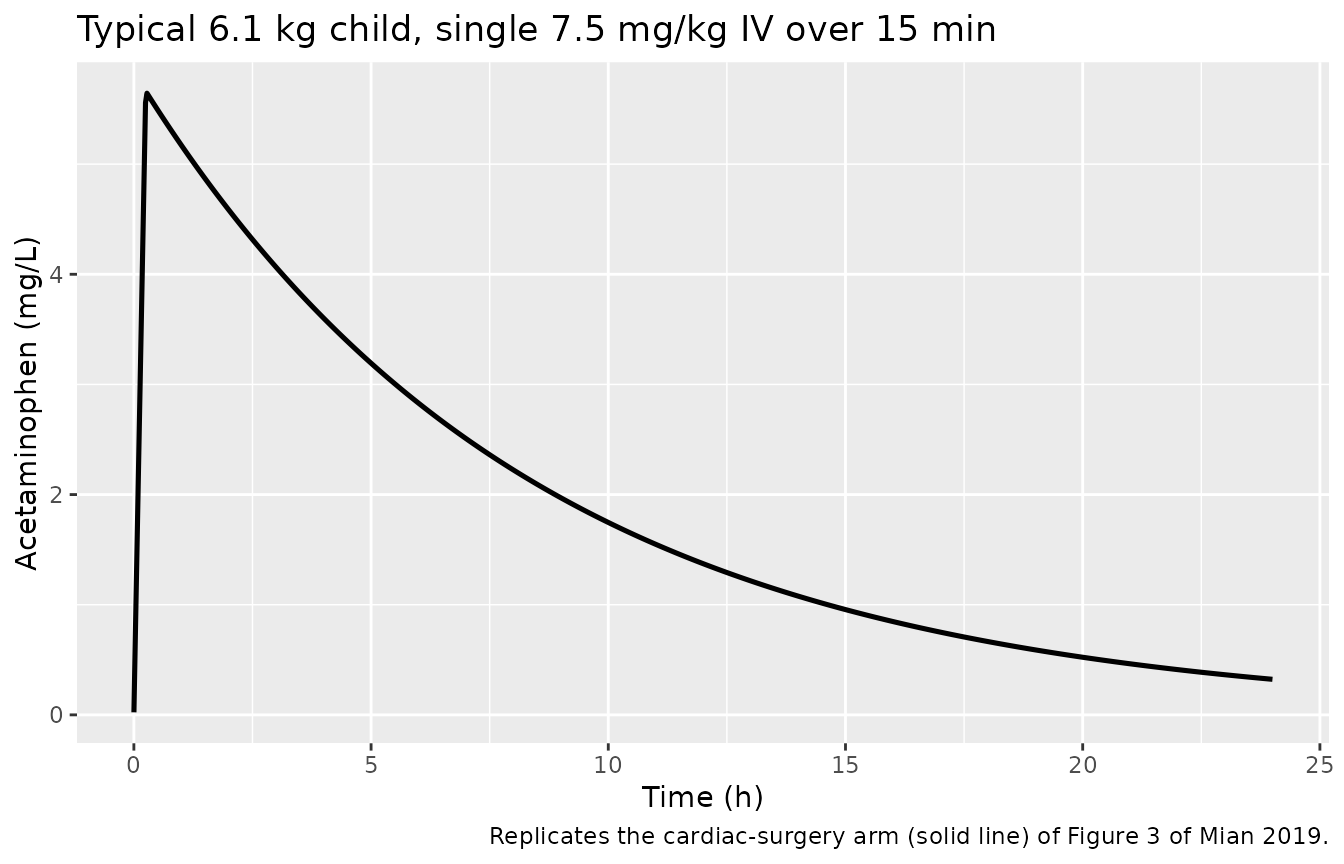
cmax_typ <- max(obs_typ$Cc)
trough_8h <- obs_typ$Cc[which.min(abs(obs_typ$time - 8))]

# Prins et al (reference 29 of Mian 2019), as quoted in the Results: CL 1.04
# L/h, central 0.69 L and peripheral 3.80 L (Vss 4.49 L) for the same 6.1 kg
# child. The inter-compartmental clearance is NOT quoted, so the comparator
# curve cannot be simulated; what CAN be tested is that the paper's "Cmax was
# 84% lower after cardiac surgery" implies a comparator Cmax that a 2-compartment
# model with those volumes can actually produce -- i.e. it must lie between
# dose/Vss (the fully-distributed lower bound) and dose/V1 (the instantaneous
# bolus upper bound).
dose_typ <- 7.5 * 6.1
implied_prins_cmax <- cmax_typ / (1 - 0.84)
prins_lower <- dose_typ / 4.49
prins_upper <- dose_typ / 0.69

stopifnot(
  implied_prins_cmax > prins_lower,
  implied_prins_cmax < prins_upper
)

tibble::tibble(
  Quantity = c(
    "Cmax, cardiac surgery (mg/L)",
    "Trough at 8 h, cardiac surgery (mg/L)",
    "Implied Cmax after non-cardiac surgery (mg/L)",
    "Lower bound, dose / Vss of Prins (mg/L)",
    "Upper bound, dose / V1 of Prins (mg/L)"
  ),
  Value = c(cmax_typ, trough_8h, implied_prins_cmax, prins_lower, prins_upper)
) |>
knitr::kable(digits = 3, caption = "Figure 3 claims. The paper states Cmax was 84% lower after cardiac surgery than after non-cardiac surgery; the implied comparator Cmax is consistent with the central and steady-state volumes it quotes for Prins et al.")| Quantity | Value |
|---|---|
| Cmax, cardiac surgery (mg/L) | 5.644 |
| Trough at 8 h, cardiac surgery (mg/L) | 2.223 |
| Implied Cmax after non-cardiac surgery (mg/L) | 35.276 |
| Lower bound, dose / Vss of Prins (mg/L) | 10.189 |
| Upper bound, dose / V1 of Prins (mg/L) | 66.304 |
Figure 1 – all four analytes over the administered three-dose regimen
Figure 1 of Mian 2019 is the structural schematic rather than a data figure. The panel below shows what that structure produces for the regimen the children actually received (three doses, 8-hour intervals), as a median with a 5th-95th percentile band across the virtual cohort.
sim_md |>
  dplyr::filter(time > 0) |>
  dplyr::select(id, time, treatment, Cc, Cc_sulf, Cc_gluc, Cc_cysmer) |>
  tidyr::pivot_longer(
    c(Cc, Cc_sulf, Cc_gluc, Cc_cysmer),
    names_to = "analyte", values_to = "conc"
  ) |>
  dplyr::mutate(
    analyte = factor(
      analyte,
      levels = c("Cc", "Cc_sulf", "Cc_gluc", "Cc_cysmer"),
      labels = c("Acetaminophen", "Sulfate", "Glucuronide", "Oxidative (cys + merc)")
    )
  ) |>
  dplyr::group_by(analyte, treatment, time) |>
  dplyr::summarise(
    Q05 = quantile(conc, 0.05),
    Q50 = median(conc),
    Q95 = quantile(conc, 0.95),
    .groups = "drop"
  ) |>
  ggplot(aes(time, Q50, colour = treatment, fill = treatment)) +
  geom_ribbon(aes(ymin = Q05, ymax = Q95), alpha = 0.2, colour = NA) +
  geom_line(linewidth = 0.8) +
  facet_wrap(~analyte, scales = "free_y", ncol = 2) +
  scale_y_log10() +
  labs(
    x = "Time (h)", y = "Concentration in acetaminophen equivalents (mg/L)",
    colour = NULL, fill = NULL,
    title = "Three 8-hourly IV doses, virtual cohort (n = 120)",
    caption = "Model structure of Figure 1 of Mian 2019, simulated over the study's dosing protocol."
  ) +
  theme(legend.position = "bottom")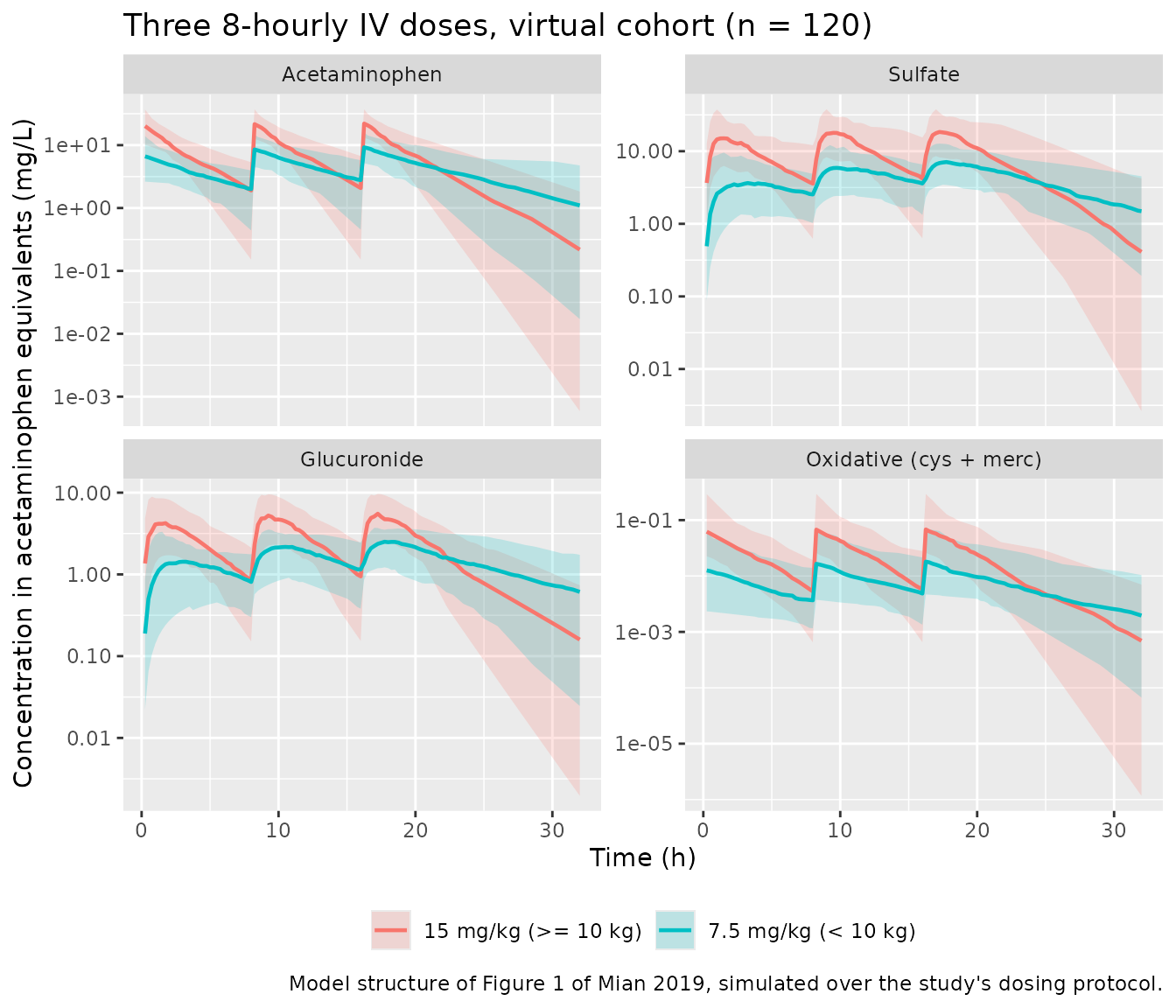
PKNCA validation
Mian 2019 reports no non-compartmental analysis, so PKNCA is used here as an independent integrator to test the model’s mass balance rather than to match a published NCA table. For a single intravenous dose the model implies four exact identities:
CL_APAP     * AUCinf(APAP)        = Dose
CLE_sulf    * AUCinf(sulfate)     = fm_sulf    * Dose
CLE_gluc    * AUCinf(glucuronide) = fm_gluc    * Dose
CLE_ox      * AUCinf(oxidative)   = fm_cysmer  * Dose
because every concentration is expressed in acetaminophen equivalents and the four pathway fractions sum to one. These hold per subject, with each subject’s own random effects.
# One PKNCA pass per analyte. Defined at the top level of the chunk so the
# helper is visible in the knit environment.
run_nca <- function(sim, analyte_col, label, dose_df = NULL) {
  conc <- sim |>
    dplyr::rename(Cc_value = dplyr::all_of(analyte_col)) |>
    # ONLY !is.na(): a `time > 0` or `Cc > 0` filter drops the time-zero row
    # that PKNCA needs to anchor AUC0-inf.
    dplyr::filter(!is.na(Cc_value)) |>
    dplyr::select(id, time, treatment, Cc = Cc_value)

  conc <- dplyr::bind_rows(
    conc,
    conc |> dplyr::distinct(id, treatment) |> dplyr::mutate(time = 0, Cc = 0)
  ) |>
    dplyr::distinct(id, treatment, time, .keep_all = TRUE) |>
    dplyr::arrange(id, treatment, time)

  if (is.null(dose_df)) {
    dose_df <- events_sd |>
      dplyr::filter(evid == 1L) |>
      dplyr::select(id, time, amt, treatment)
  }

  conc_obj <- PKNCA::PKNCAconc(conc, Cc ~ time | treatment + id, concu = "mg/L", timeu = "h")
  dose_obj <- PKNCA::PKNCAdose(dose_df, amt ~ time | treatment + id, doseu = "mg")

  intervals <- data.frame(
    start = 0, end = Inf,
    cmax = TRUE, tmax = TRUE, aucinf.obs = TRUE, half.life = TRUE
  )

  res <- suppressWarnings(
    PKNCA::pk.nca(PKNCA::PKNCAdata(conc_obj, dose_obj, intervals = intervals))
  )
  as.data.frame(res$result) |> dplyr::mutate(analyte = label)
}

nca_all <- dplyr::bind_rows(
  run_nca(sim_sd, "Cc", "Acetaminophen"),
  run_nca(sim_sd, "Cc_sulf", "Sulfate"),
  run_nca(sim_sd, "Cc_gluc", "Glucuronide"),
  run_nca(sim_sd, "Cc_cysmer", "Oxidative (cys + merc)")
)

stopifnot(nrow(nca_all) > 0, !all(is.na(nca_all$PPORRES)))
nca_all |>
  dplyr::filter(PPTESTCD %in% c("cmax", "tmax", "aucinf.obs", "half.life")) |>
  dplyr::group_by(analyte, treatment, PPTESTCD) |>
  dplyr::summarise(
    Median = median(PPORRES, na.rm = TRUE),
    P05 = quantile(PPORRES, 0.05, na.rm = TRUE),
    P95 = quantile(PPORRES, 0.95, na.rm = TRUE),
    .groups = "drop"
  ) |>
  dplyr::mutate(Parameter = nlmixr2lib::ncaParamLabel(PPTESTCD)) |>
  dplyr::select(analyte, treatment, Parameter, Median, P05, P95) |>
  dplyr::rename(
    "Analyte" = analyte,
    "Dose band" = treatment,
    "NCA parameter" = Parameter,
    "5th pct" = P05,
    "95th pct" = P95
  ) |>
  knitr::kable(
    digits = 3,
    caption = "Simulated single-dose NCA by analyte and dose band (virtual cohort, n = 120). Mian 2019 reports no NCA values, so there is no published column to compare against."
)| Analyte | Dose band | NCA parameter | Median | 5th pct | 95th pct |
|---|---|---|---|---|---|
| Acetaminophen | 15 mg/kg (>= 10 kg) | AUC0-∞ (obs) | 85.742 | 51.496 | 154.090 |
| Acetaminophen | 15 mg/kg (>= 10 kg) | Cmax | 17.903 | 11.689 | 30.044 |
| Acetaminophen | 15 mg/kg (>= 10 kg) | t½ | 3.036 | 1.037 | 7.609 |
| Acetaminophen | 15 mg/kg (>= 10 kg) | Tmax | 0.273 | 0.273 | 0.273 |
| Acetaminophen | 7.5 mg/kg (< 10 kg) | AUC0-∞ (obs) | 49.256 | 22.566 | 101.917 |
| Acetaminophen | 7.5 mg/kg (< 10 kg) | Cmax | 5.981 | 2.492 | 13.740 |
| Acetaminophen | 7.5 mg/kg (< 10 kg) | t½ | 5.127 | 1.596 | 19.878 |
| Acetaminophen | 7.5 mg/kg (< 10 kg) | Tmax | 0.273 | 0.273 | 0.273 |
| Glucuronide | 15 mg/kg (>= 10 kg) | AUC0-∞ (obs) | 26.837 | 19.247 | 59.937 |
| Glucuronide | 15 mg/kg (>= 10 kg) | Cmax | 3.829 | 1.449 | 10.131 |
| Glucuronide | 15 mg/kg (>= 10 kg) | t½ | 3.057 | 1.038 | 7.615 |
| Glucuronide | 15 mg/kg (>= 10 kg) | Tmax | 2.000 | 0.624 | 4.275 |
| Glucuronide | 7.5 mg/kg (< 10 kg) | AUC0-∞ (obs) | 17.890 | 9.931 | 36.587 |
| Glucuronide | 7.5 mg/kg (< 10 kg) | Cmax | 1.463 | 0.483 | 3.218 |
| Glucuronide | 7.5 mg/kg (< 10 kg) | t½ | 5.475 | 1.887 | 20.296 |
| Glucuronide | 7.5 mg/kg (< 10 kg) | Tmax | 3.250 | 1.000 | 11.500 |
| Oxidative (cys + merc) | 15 mg/kg (>= 10 kg) | AUC0-∞ (obs) | 0.190 | 0.028 | 0.447 |
| Oxidative (cys + merc) | 15 mg/kg (>= 10 kg) | Cmax | 0.043 | 0.006 | 0.148 |
| Oxidative (cys + merc) | 15 mg/kg (>= 10 kg) | t½ | 3.036 | 1.037 | 7.609 |
| Oxidative (cys + merc) | 15 mg/kg (>= 10 kg) | Tmax | 0.273 | 0.273 | 0.273 |
| Oxidative (cys + merc) | 7.5 mg/kg (< 10 kg) | AUC0-∞ (obs) | 0.114 | 0.027 | 0.414 |
| Oxidative (cys + merc) | 7.5 mg/kg (< 10 kg) | Cmax | 0.015 | 0.002 | 0.092 |
| Oxidative (cys + merc) | 7.5 mg/kg (< 10 kg) | t½ | 5.127 | 1.596 | 19.878 |
| Oxidative (cys + merc) | 7.5 mg/kg (< 10 kg) | Tmax | 0.273 | 0.273 | 0.273 |
| Sulfate | 15 mg/kg (>= 10 kg) | AUC0-∞ (obs) | 64.253 | 38.971 | 136.910 |
| Sulfate | 15 mg/kg (>= 10 kg) | Cmax | 11.264 | 4.160 | 19.078 |
| Sulfate | 15 mg/kg (>= 10 kg) | t½ | 3.036 | 1.411 | 7.641 |
| Sulfate | 15 mg/kg (>= 10 kg) | Tmax | 1.500 | 0.694 | 3.075 |
| Sulfate | 7.5 mg/kg (< 10 kg) | AUC0-∞ (obs) | 52.947 | 28.533 | 118.401 |
| Sulfate | 7.5 mg/kg (< 10 kg) | Cmax | 4.366 | 1.379 | 13.124 |
| Sulfate | 7.5 mg/kg (< 10 kg) | t½ | 5.400 | 1.852 | 22.126 |
| Sulfate | 7.5 mg/kg (< 10 kg) | Tmax | 3.250 | 1.000 | 11.750 |
Mass-balance recovery – typical values
The identity is exact in the model, so the deterministic typical-value solve is where it can be asserted tightly: any residual here is purely PKNCA’s trapezoidal and lambda-z extrapolation error on a noise-free profile.
fm <- c(
  "Acetaminophen" = 1.00,
  "Sulfate" = 0.49,
  "Glucuronide" = 0.36,
  "Oxidative (cys + merc)" = 0.10
)
analyte_col <- c(
  "Acetaminophen" = "Cc", "Sulfate" = "Cc_sulf",
  "Glucuronide" = "Cc_gluc", "Oxidative (cys + merc)" = "Cc_cysmer"
)
clearance_col <- c(
  "Acetaminophen" = "cl", "Sulfate" = "cle_sulf",
  "Glucuronide" = "cle_gluc", "Oxidative (cys + merc)" = "cle_cysmer"
)

typ_dose <- 7.5 * 6.1
typ_nca_events <- dplyr::bind_rows(
  tibble::tibble(
    id = 1L, WT = 6.1, treatment = "typical 6.1 kg", time = 0, evid = 1L,
    amt = typ_dose, rate = typ_dose / 0.25, cmt = "central"
  ),
  tibble::tibble(
    id = 1L, WT = 6.1, treatment = "typical 6.1 kg", time = obs_times,
    evid = 0L, amt = NA_real_, rate = NA_real_, cmt = "Cc"
  )
) |>
  dplyr::arrange(time, dplyr::desc(evid))

sim_typ_nca <- rxode2::rxSolve(
  mod_typ, typ_nca_events,
  omega = NA, useLinCmt = FALSE, maxsteps = 1e5, atol = 1e-12, rtol = 1e-10
) |>
  as.data.frame() |>
  dplyr::mutate(treatment = "typical 6.1 kg")

# rxSolve omits the `id` column entirely for a single-subject event table;
# restore it so the PKNCA grouping formula below has something to group on.
if (is.null(sim_typ_nca$id)) sim_typ_nca$id <- 1L

typ_dose_df <- tibble::tibble(id = 1L, time = 0, amt = typ_dose, treatment = "typical 6.1 kg")

recovery_typ <- do.call(dplyr::bind_rows, lapply(names(fm), function(a) {
  nca <- run_nca(sim_typ_nca, analyte_col[[a]], a, dose_df = typ_dose_df)
  auc <- nca$PPORRES[nca$PPTESTCD == "aucinf.obs"]
  tibble::tibble(
    analyte = a,
    recovery = unique(sim_typ_nca[[clearance_col[[a]]]]) * auc / (fm[[a]] * typ_dose)
  )
}))

# Deterministic profile, so the tolerance is the integrator's, not the
# cohort's: observed |recovery - 1| was <= 7e-5 for every analyte.
stopifnot(
  nrow(recovery_typ) == length(fm),
  !anyNA(recovery_typ$recovery),
  max(abs(recovery_typ$recovery - 1)) < 0.002
)

recovery_typ |>
  dplyr::mutate(`Deviation (%)` = 100 * (recovery - 1)) |>
  dplyr::rename("Analyte" = analyte, "Recovery" = recovery) |>
knitr::kable(digits = c(0, 6, 4), caption = "Typical 6.1 kg child, single 7.5 mg/kg dose: clearance x AUC0-inf divided by the dose routed down that pathway.")| Analyte | Recovery | Deviation (%) |
|---|---|---|
| Acetaminophen | 0.999958 | -0.0042 |
| Sulfate | 0.999876 | -0.0124 |
| Glucuronide | 0.999929 | -0.0071 |
| Oxidative (cys + merc) | 0.999957 | -0.0043 |
Mass-balance recovery – across the virtual cohort
The same identity holds subject by subject, with each subject’s own random effects. Assertions here are on the centre and on robust quantiles rather than on the extremes, because the extreme of a random cohort is not reproducible across rxode2 builds or solver-thread counts.
subj_par <- sim_sd |>
  dplyr::distinct(id, treatment, cl, cle_sulf, cle_gluc, cle_cysmer)

dose_by_id <- events_sd |>
  dplyr::filter(evid == 1L) |>
  dplyr::select(id, dose = amt)

recovery <- nca_all |>
  dplyr::filter(PPTESTCD == "aucinf.obs") |>
  dplyr::select(id, treatment, analyte, aucinf = PPORRES) |>
  dplyr::left_join(subj_par, by = c("id", "treatment")) |>
  dplyr::left_join(dose_by_id, by = "id") |>
  dplyr::mutate(
    clearance = dplyr::case_when(
      analyte == "Acetaminophen" ~ cl,
      analyte == "Sulfate" ~ cle_sulf,
      analyte == "Glucuronide" ~ cle_gluc,
      TRUE ~ cle_cysmer
    ),
    fraction = unname(fm[analyte]),
    recovery = clearance * aucinf / (fraction * dose),
    dev = abs(recovery - 1)
  )

stopifnot(nrow(recovery) == n_sub * length(fm), !anyNA(recovery$recovery))

recovery_summary <- recovery |>
  dplyr::group_by(analyte) |>
  dplyr::summarise(
    `Median recovery` = median(recovery),
    `75th pct |dev| (%)` = 100 * quantile(dev, 0.75),
    `90th pct |dev| (%)` = 100 * quantile(dev, 0.90),
    `Max |dev| (%)` = 100 * max(dev),
    .groups = "drop"
  )

# Realised across two seeds and 1 / 4 solver threads: median deviation
# <= 3e-4 for every analyte; 75th percentile <= 0.10%; 90th percentile
# <= 0.29%. The bounds below sit well outside that spread and still fail
# instantly on a mis-specified pathway fraction or clearance, which moves
# the median by tens of percent. The MAXIMUM is deliberately not gated: it
# is dominated by the handful of subjects discussed below whose metabolite
# terminal phase is unresolved in a 36 h window, and the extreme of a
# random cohort is not reproducible across builds.
stopifnot(
  max(abs(recovery_summary$`Median recovery` - 1)) < 0.005,
  max(recovery_summary$`75th pct |dev| (%)`) < 2,
  max(recovery_summary$`90th pct |dev| (%)`) < 2,
  # Parent and oxidative pool are mono-exponential well inside the window,
  # so those two are tight even at the extreme.
  max(dplyr::filter(recovery, analyte %in% c("Acetaminophen", "Oxidative (cys + merc)"))$dev) < 0.01
)

recovery_summary |>
  dplyr::rename("Analyte" = analyte) |>
knitr::kable(digits = c(0, 5, 3, 3, 3), caption = "Mass balance across the virtual cohort: clearance x AUC0-inf divided by the dose routed down that pathway.")| Analyte | Median recovery | 75th pct |dev| (%) | 90th pct |dev| (%) | Max |dev| (%) |
|---|---|---|---|---|
| Acetaminophen | 0.99994 | 0.009 | 0.012 | 0.027 |
| Glucuronide | 0.99971 | 0.071 | 0.245 | 103.407 |
| Oxidative (cys + merc) | 0.99994 | 0.009 | 0.012 | 0.027 |
| Sulfate | 0.99976 | 0.072 | 0.207 | 23.127 |
A small minority of subjects draw a sulfate or glucuronide
elimination rate constant close to the parent’s, which makes the
metabolite profile nearly t * exp(-k t); its log-linear
slope then approaches the true terminal rate only asymptotically, and
PKNCA’s automatic lambda-z window over-extrapolates
AUC0-inf within a 36-hour sampling window. Extending the
window shrinks those outliers monotonically (the 90th-percentile
deviation falls from 0.25% at 36 h to 0.16% at 42 h) at the cost of
pushing the fastest subjects’ oxidative pool into solver noise. This is
a property of the NCA estimator, not of the model: the deterministic
gate above reproduces the identity to better than 1e-4.
# Prove the gate is not vacuous. Note first WHAT it can and cannot detect:
# perturbing a metabolite's own elimination clearance or volume leaves
# `CLE * AUC0-inf` invariant, because the AUC moves inversely with the
# clearance -- the identity is structural. What the gate does detect is a
# wrong PATHWAY FRACTION, which is exactly the load-bearing assumption of
# this model (the fm values were fixed from the literature, not estimated).
#
# Doubling fm_sulf to 0.98 leaves the other three fractions alone, so the
# parent's total elimination becomes (0.98 + 0.51) * kel and the share of
# dose reaching sulfate becomes 0.98 / 1.49 = 0.658. Scored against the
# published 0.49 the recovery must be 0.98 / (1.49 * 0.49) = 1.342.
mod_mut <- rxode2::ini(mod_typ, fm_sulf = 0.49 * 2)
#> ℹ change initial estimate of `fm_sulf` to `0.98`

sulf_recovery <- function(model) {
  s <- rxode2::rxSolve(
    model, typ_nca_events,
    omega = NA, useLinCmt = FALSE, maxsteps = 1e5, atol = 1e-12, rtol = 1e-10
  ) |>
    as.data.frame() |>
    dplyr::mutate(treatment = "typical 6.1 kg")
  if (is.null(s$id)) s$id <- 1L
  nca <- run_nca(s, "Cc_sulf", "Sulfate", dose_df = typ_dose_df)
  auc <- nca$PPORRES[nca$PPTESTCD == "aucinf.obs"]
  unique(s$cle_sulf) * auc / (0.49 * typ_dose)
}

rec_base <- sulf_recovery(mod_typ)
rec_mut <- sulf_recovery(mod_mut)

stopifnot(
  abs(rec_base - 1) < 0.002, # the correct model passes
  abs(rec_mut - 0.98 / (1.49 * 0.49)) < 0.01 # the mutated model lands where it must
)

tibble::tibble(
  Model = c("As published (fm_sulf = 0.49)", "Mutated (fm_sulf = 0.98)"),
  `Sulfate recovery` = c(rec_base, rec_mut),
  `Expected` = c(1, 0.98 / (1.49 * 0.49))
) |>
knitr::kable(digits = 4, caption = "Mutation control: doubling the assumed sulfation fraction moves the mass-balance gate by 34%, so the gate is not vacuous.")| Model | Sulfate recovery | Expected |
|---|---|---|
| As published (fm_sulf = 0.49) | 0.9999 | 1.0000 |
| Mutated (fm_sulf = 0.98) | 1.3418 | 1.3423 |
Metabolite exposure shares
A second, independent consequence of the fixed formation fractions is
that each metabolite’s AUC-weighted mass share of the dose must equal
its fm.
shares <- recovery |>
  dplyr::filter(analyte != "Acetaminophen") |>
  dplyr::mutate(mass_recovered = clearance * aucinf / dose) |>
  dplyr::group_by(analyte) |>
  dplyr::summarise(
    `Assumed fm` = unique(fraction),
    `Median recovered fraction of dose` = median(mass_recovered),
    .groups = "drop"
  )

stopifnot(max(abs(shares$`Median recovered fraction of dose` - shares$`Assumed fm`) / shares$`Assumed fm`) < 0.01)

shares |>
knitr::kable(digits = 4, caption = "Fraction of the administered acetaminophen dose recovered through each metabolite pathway, against the literature fractions the authors fixed (Methods).")| analyte | Assumed fm | Median recovered fraction of dose |
|---|---|---|
| Glucuronide | 0.36 | 0.3599 |
| Oxidative (cys + merc) | 0.10 | 0.1000 |
| Sulfate | 0.49 | 0.4899 |
Assumptions and deviations
Weight distribution. The paper reports only the median (6.1 kg) and range (4.0-12.9 kg) of body weight. The virtual cohort spreads weight uniformly over that range, which is a deliberate choice for covariate coverage rather than a claim about the trial’s weight distribution.
Dosing band. The protocol gives 7.5 mg/kg below 10 kg and 15 mg/kg at or above 10 kg. That rule is applied to the simulated weights, so the cohort splits into two dose bands. The paper’s typical-value figure (Figure 3) uses a single 7.5 mg/kg dose in a 6.1-kg child, which is reproduced separately.
The linear weight model is not extrapolable. Because the clearances are linear in weight with a negative intercept,
CLE_APAPreaches zero at about 2.2 kg and is negative below it. The authors state explicitly that extrapolation outside the studied 4.0-12.9 kg range is not justified. All simulations here stay inside that range, and the weight identity chunk asserts every clearance remains positive.Centred versus printed weight equation. The model file stores the centred form
CLE = CLE_6.1 + theta_slope * (BW/6.1 - 1)instead of Table 2’s printedCLE = theta_slope * (BW/6.1) + theta_intercept. The two are algebraically identical; the identity is asserted to better than 1e-10 L/h at six weights spanning the studied range, andtheta_slopeis stored verbatim. This keeps the canonicallcl/lcle_*names meaning “typical clearance at the reference weight”, and makes the parent value the paper’s own headline figure of 0.96 L/h.Residual error scale. Table 2’s residual-variability block is headed
[sigma^2], so the printed values are variances and the nlmixr2 proportional SD is their square root (0.382, 0.225, 0.285, 0.222). The Results text adds “the residual variability was generally well below 15%”, which is inconsistent with that reading; the most likely referent is the RSE column of the same block (29%, 15%, 14%, 12%). The table header is the machine-readable statement and is what the model follows.Metabolite parameters are conditional on the assumed fractions. The authors fixed the formation fractions (0.49 sulfation, 0.36 glucuronidation, 0.10 oxidation, 0.05 unchanged) from the literature because the metabolite sub-model is otherwise unidentifiable, and warn that “absolute values of the parameters related to the metabolites should be considered only in the context of the assumptions made”. The combined oxidative pool in particular carries a very small volume (0.042 L) and a very large elimination clearance (39.6 L/h at 6.1 kg); the product is well determined by the data but the individual values are not physiologically interpretable on their own.
Oxidative metabolites are lumped. Acetaminophen cysteine and acetaminophen mercapturate are modelled as one compartment sharing a distribution volume, following the paper. Acetaminophen glutathione was below the limit of quantification in every sample and is absent from the model.
The non-cardiac comparator in Figure 3 is not simulated. The paper quotes Prins et al only as CL = 1.04 L/h with central 0.69 L and peripheral 3.80 L; the inter-compartmental clearance is not given, so the two-compartment comparator curve cannot be reconstructed. The vignette instead tests that the paper’s “84% lower Cmax” claim implies a comparator Cmax lying between
dose / Vssanddose / V1for those volumes, which it does.The “factor 50” trough claim is not reproduced and is not gated. The Results state that the 8-hour trough was “more than a factor 50 higher” after cardiac surgery. With CL = 1.04 L/h and Vss = 4.49 L, a two-compartment comparator cannot fall from its peak to 1/50 of this model’s 8-hour trough regardless of the unreported inter-compartmental clearance, because its terminal rate constant is bounded by CL/Vss. The claim is recorded here as a documented disagreement rather than being tested; no model value was changed to accommodate it.
Screened-but-excluded covariates. Age, sex, Down syndrome, cardiopulmonary bypass time and RACHS-1 category were all tested and none was retained. They are recorded in the model’s
covariatesDataExcludedmetadata so the covariate screen is visible, but they do not appear inmodel().No non-paper-derived parameter values. Every
ini()entry traces to Table 2 or to the Methods section of Mian 2019; nothing was digitised from a figure, supplied by correspondence, or carried from an upstream model.