Bedaquiline mycobacterial-load PD model (Svensson 2017)
Source:vignettes/articles/Svensson_2017_bedaquiline.Rmd
Svensson_2017_bedaquiline.RmdModel and source
ui <- rxode2::rxode(readModelDb("Svensson_2017_bedaquiline"))
#> ℹ parameter labels from comments will be replaced by 'label()'- Citation: Svensson E. M., Karlsson M. O. (2017). Modelling of mycobacterial load reveals bedaquiline’s exposure-response relationship in patients with drug-resistant TB. Journal of Antimicrobial Chemotherapy 72(12):3398-3405. doi:10.1093/jac/dkx317. Bedaquiline weekly-average plasma concentration CAV is computed from the upstream population PK model of Svensson E. M., Dosne A.-G., Karlsson M. O. (2016). Population pharmacokinetics of bedaquiline and metabolite M2 in drug-resistant tuberculosis patients - the effect of time-varying weight and albumin. CPT Pharmacometrics Syst Pharmacol 5(12):682-691. doi:10.1002/psp4.12147; see modellib(‘Svensson_2016_bedaquiline’). Box-Cox-transformed IIV distribution follows Petersson K. J. F., Hanze E., Savic R. M. et al. (2009). Semiparametric distributions with estimated shape parameters. Pharm Res 26(9):2174-2185. doi:10.1007/s11095-009-9931-1.
- Description: Pharmacodynamic exposure-response model for the mycobacterial load (MBL, n bacteria per sample inoculum) in adult patients with drug-resistant pulmonary tuberculosis treated with bedaquiline plus an optimized background regimen. The latent MBL state declines mono-exponentially with a half-life HL that is prolonged by 28.1% in patients with pre-XDR or XDR tuberculosis and shortened by individual bedaquiline weekly-average plasma concentration CAV via an Emax model with the maximum fractional effect on HL fixed at -100% (EC50 1.42 mg/L). The per-subject starting MBL_0 is informed by the baseline mean Time-to-Positivity in MGIT liquid culture (TTP_MGIT_BASE) via a power-form covariate (exponent -3.69 around the cohort median 6.8 days). Inter-individual variability on log HL uses a Box-Cox-transformed eta distribution (Petersson 2009 form, shape 0.66, variance 0.33); inter-occasion variability in sputum sampling on log MBL (variance 3.71) is folded into the residual log-scale error. The Svensson 2017 source’s full 3-component model (longitudinal MBL plus per-sample probability of bacterial presence plus MGIT-tube logistic-growth-driven time-to-event for observed TTP) is reduced here to the MBL component, with the latent MBL state treated directly as the observable; the probability-of-presence and tube-growth-driven TTP machinery are measurement-model artifacts of how MBL was inferred from TTP data and are dropped (see vignette Assumptions and deviations). Bedaquiline CAV is supplied as a time-varying covariate column from any popPK source; the upstream popPK paper (Svensson 2016 CPT PSP, reference 21) is shipped in nlmixr2lib as modellib(‘Svensson_2016_bedaquiline’).
- Article: https://doi.org/10.1093/jac/dkx317
- Upstream PK paper (Svensson 2016): https://doi.org/10.1002/psp4.12147 (shipped as
modellib('Svensson_2016_bedaquiline')in nlmixr2lib) - IIV-shape reference (Petersson 2009): https://doi.org/10.1007/s11095-009-9931-1
Population
The Svensson 2017 PD dataset comes from the TMC207-C208 phase IIb
registration trial (ClinicalTrials.gov NCT00449644) sponsored by Janssen
Pharmaceuticals: 189 adult patients (median age 33 years, range 18-63;
median weight 54 kg, range 35-83; 34.5% female; 14.6% HIV-positive;
91.7% with lung cavitation) with newly diagnosed pulmonary
multidrug-resistant tuberculosis (MDR-TB), enrolled in two stages and
treated with bedaquiline 400 mg once daily for 2 weeks loading then 200
mg three times weekly for 22 weeks (active arm; n = 91) or matching
placebo (n = 98), plus an optimized background regimen of five
second-line anti-TB drugs (kanamycin, ofloxacin, ethionamide,
pyrazinamide, terizidone). TB drug-resistance type at baseline:
drug-susceptible 3.86%, MDR 46.4%, pre-XDR 25.1%, XDR 5.31%, missing
18.9% (assigned to MDR per Results paragraph 4). The pooled
DIS_TB_XDR = 1 stratum (pre-XDR + XDR) is 30.4% of the
cohort.
Microbiological sampling collected triplicate spot sputum samples the
day before treatment start, weekly until week 8, every second week until
week 24, and at ten points across the 96-week follow-up. Mycobacterial
growth indicator tube (MGIT) liquid cultures recorded the
time-to-positivity (TTP) in hours; the per-subject baseline mean TTP
(TTP_MGIT_BASE, median 6.8 days, range 2.3-42 in the n =
191 with baseline data) was used as a covariate driving the starting
mycobacterial load.
The same information is available programmatically via
ui$meta$population (after
ui <- rxode2::rxode(readModelDb("Svensson_2017_bedaquiline"))).
Source trace
| Equation / parameter | Value | Source location |
|---|---|---|
lmbl0 MBL_0 (typical) |
2.14e3 n bacteria/inoculum | Svensson 2017 Table 2 |
e_ttp_mbl0 baseline-TTP power exponent on MBL_0 |
-3.69 (95% CI -4.15 to -3.30) | Svensson 2017 Table 2 |
lhl typical half-life of MBL decline |
0.81 weeks (95% CI 0.71-0.93) | Svensson 2017 Table 2 |
e_xdr_hl pre-XDR/XDR effect on HL |
+28.1% (95% CI 9.1-51.5) | Svensson 2017 Table 2 |
lec50_bdq bedaquiline EC50 for HL effect |
1.42 mg/L (95% CI 1.00-2.05) | Svensson 2017 Table 2 |
emax_bdq bedaquiline maximum effect on HL |
1 FIX (= -100%) | Svensson 2017 Table 2 |
lambda_bc Box-Cox shape |
0.66 (95% CI 0.34-1.05) | Svensson 2017 Table 2 |
etalhl IIV on log HL (variance) |
0.33 (95% CI 0.25-0.45) | Svensson 2017 Table 2 |
expSd_MBL residual log-scale SD (= sqrt of IOV_sputum
variance) |
1.926 = sqrt(3.71) | Svensson 2017 Table 2 (IOV_sputum variance 3.71, 95% CI 3.29-4.38) |
| Equation 1 (MBL_i(TAST) = MBL_0 * (mTTP_0_i/mTTP_0_p)^COVTTP * exp(-ln(2)/HL_i * TAST)) | n/a | Svensson 2017 Equation 1, page 3400 |
| Bedaquiline Emax form on HL (HL_i = HL_typ * EC50/(EC50+CAV) at emax = 1) | n/a | Svensson 2017 Results ‘Covariate and PK effects’, page 3401 |
| Box-Cox transformation form (eta_BC = (exp(eta)^lambda - 1)/lambda) | n/a | Petersson 2009 (reference 29 of Svensson 2017); same NM-TRAN form
translated by Schoemaker_2018_levetiracetam.R
|
The probability-of-bacterial-presence model (Equation 2) and the MGIT-tube logistic growth + TTP time-to-event model (Equation 3) of the source’s full 3-component analysis are intentionally omitted from this extraction; only the underlying mycobacterial-load decline (Equation 1) is implemented, with the latent MBL state treated directly as the observable. See the Assumptions and deviations section below for the rationale.
Virtual cohort
Original observed data are not publicly redistributable. The
simulation below builds typical-value cohorts for four
bedaquiline-exposure scenarios crossed with two TB drug-resistance
strata (MDR vs pre-XDR/XDR), mirroring the eight scenarios reported in
Svensson 2017 Table 3 and Figure 4. Exposure scenarios use constant
CAV (the time-varying loading-vs-maintenance schedule is
held flat for illustration; see Assumptions and deviations).
The median observed weekly-average bedaquiline concentration is
approximately 1.5 mg/L at week 2 (derived from the Svensson 2017 Results
‘Covariate and PK effects’ paragraph: at the 50th percentile exposure
the typical half-life is 51.6% shorter than placebo, implying
CAV / (1.42 + CAV) = 0.516,
i.e. CAV ~ 1.5 mg/L).
set.seed(20170917)

t_obs_weeks <- seq(0, 24, by = 0.5)  # weekly observations until week 24

make_cohort <- function(n, cav_mgL, xdr, scenario_label,
                        ttp_base_days = 6.8, id_offset = 0L) {
  ids <- id_offset + seq_len(n)
  expand.grid(id = ids, time = t_obs_weeks) |>
    dplyr::arrange(id, time) |>
    dplyr::mutate(
      evid          = 0L,
      amt           = 0,
      CAV           = cav_mgL,
      DIS_TB_XDR    = xdr,
      TTP_MGIT_BASE = ttp_base_days,
      scenario      = scenario_label
    )
}

n_per_scenario <- 100L

events <- dplyr::bind_rows(
  make_cohort(n_per_scenario, cav_mgL = 0.00, xdr = 0L,
              scenario_label = "MDR + placebo",                       id_offset =   0L),
  make_cohort(n_per_scenario, cav_mgL = 0.75, xdr = 0L,
              scenario_label = "MDR + low BDQ (CAV 0.75 mg/L)",       id_offset = 100L),
  make_cohort(n_per_scenario, cav_mgL = 1.50, xdr = 0L,
              scenario_label = "MDR + median BDQ (CAV 1.50 mg/L)",    id_offset = 200L),
  make_cohort(n_per_scenario, cav_mgL = 3.00, xdr = 0L,
              scenario_label = "MDR + high BDQ (CAV 3.00 mg/L)",      id_offset = 300L),
  make_cohort(n_per_scenario, cav_mgL = 0.00, xdr = 1L,
              scenario_label = "pre-XDR/XDR + placebo",               id_offset = 400L),
  make_cohort(n_per_scenario, cav_mgL = 0.75, xdr = 1L,
              scenario_label = "pre-XDR/XDR + low BDQ (CAV 0.75 mg/L)",   id_offset = 500L),
  make_cohort(n_per_scenario, cav_mgL = 1.50, xdr = 1L,
              scenario_label = "pre-XDR/XDR + median BDQ (CAV 1.50 mg/L)",id_offset = 600L),
  make_cohort(n_per_scenario, cav_mgL = 3.00, xdr = 1L,
              scenario_label = "pre-XDR/XDR + high BDQ (CAV 3.00 mg/L)",  id_offset = 700L)
)

stopifnot(!anyDuplicated(unique(events[, c("id", "time", "evid")])))
nrow(events)
#> [1] 39200
length(unique(events$id))
#> [1] 800
Simulation
mod_full <- rxode2::rxode(readModelDb("Svensson_2017_bedaquiline"))
#> ℹ parameter labels from comments will be replaced by 'label()'

# Typical-value simulation (Svensson 2017 Figure 4 shows typical impact of bedaquiline
# exposure, not VPCs). zeroRe() drops the Box-Cox-transformed eta on log HL and the
# log-scale residual error so each id traces the typical trajectory for its scenario.
mod_typ <- mod_full |> rxode2::zeroRe()

sim_typ <- rxode2::rxSolve(
  mod_typ,
  events = events,
  keep   = c("scenario", "CAV", "DIS_TB_XDR", "TTP_MGIT_BASE")
) |>
  as.data.frame()
#> ℹ omega/sigma items treated as zero: 'etalhl'
#> Warning: multi-subject simulation without without 'omega'
# Stochastic VPC-style simulation: keep IIV + residual error in place. Used for
# the percentile-band figure below.
sim_stoch <- rxode2::rxSolve(
  mod_full,
  events = events,
  keep   = c("scenario", "CAV", "DIS_TB_XDR", "TTP_MGIT_BASE")
) |>
  as.data.frame()
Replicate published figures
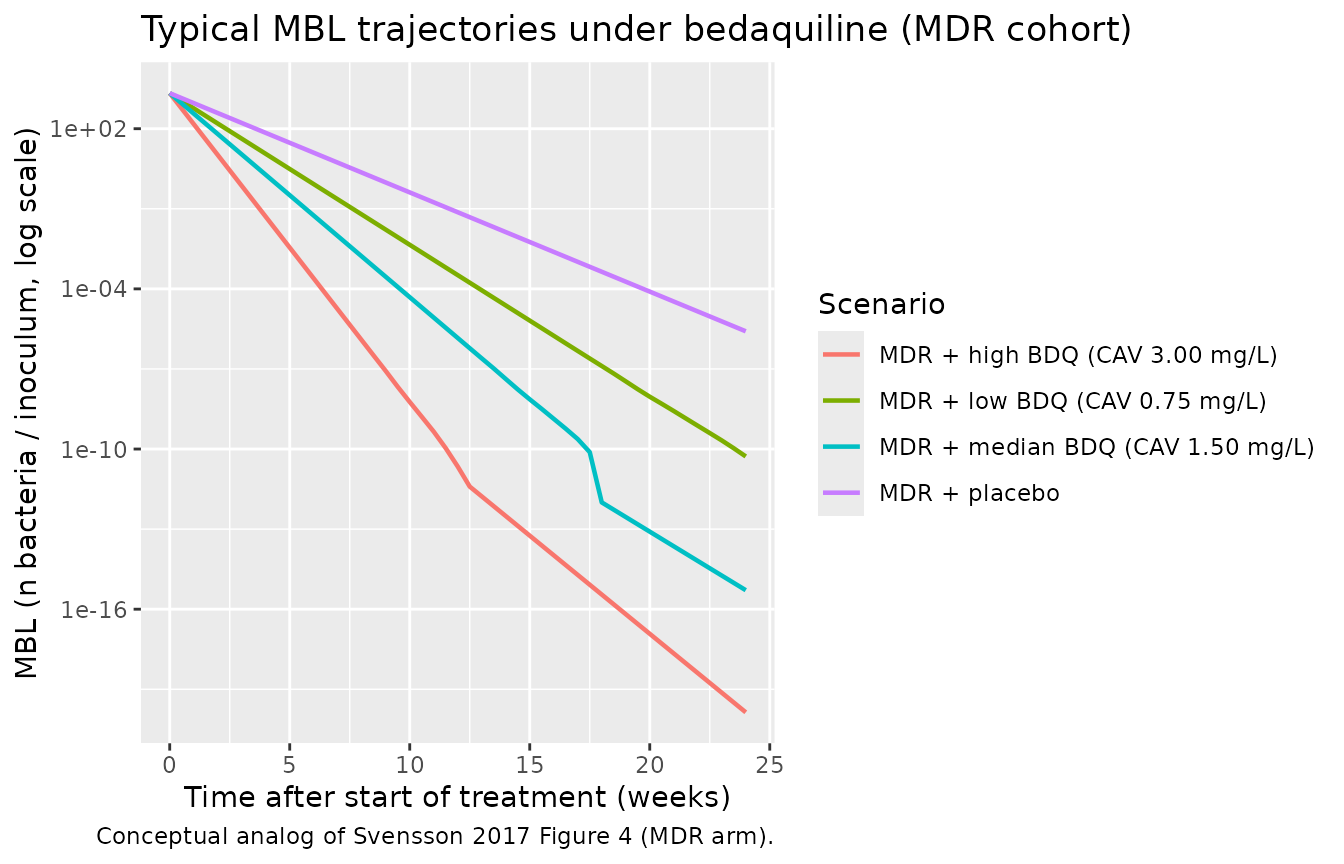
MBL trajectories by bedaquiline exposure (MDR cohort)
# Conceptual analog of Svensson 2017 Figure 4: typical-value MBL trajectories
# over 24 weeks of treatment, stratified by bedaquiline exposure scenario for
# MDR patients. The source's Figure 4 plots "proportion of patients without
# SCC" -- a TTE-derived metric -- rather than the underlying MBL state; this
# vignette plots MBL directly because the TTE / probability-of-presence
# measurement model is not extracted (see Assumptions and deviations).
sim_typ |>
  dplyr::filter(DIS_TB_XDR == 0L) |>
  dplyr::distinct(time, scenario, MBL) |>
  ggplot(aes(time, MBL, color = scenario)) +
  geom_line(linewidth = 0.8) +
  scale_y_log10() +
  labs(
    x        = "Time after start of treatment (weeks)",
    y        = "MBL (n bacteria / inoculum, log scale)",
    color    = "Scenario",
    title    = "Typical MBL trajectories under bedaquiline (MDR cohort)",
    caption  = "Conceptual analog of Svensson 2017 Figure 4 (MDR arm)."
  )
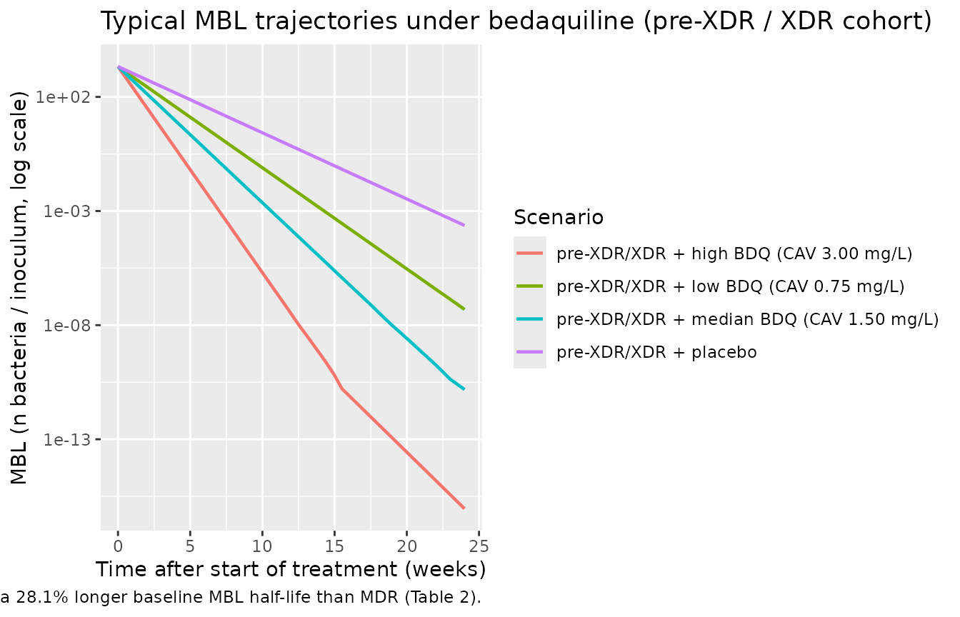
MBL trajectories by bedaquiline exposure (pre-XDR / XDR cohort)
sim_typ |>
  dplyr::filter(DIS_TB_XDR == 1L) |>
  dplyr::distinct(time, scenario, MBL) |>
  ggplot(aes(time, MBL, color = scenario)) +
  geom_line(linewidth = 0.8) +
  scale_y_log10() +
  labs(
    x        = "Time after start of treatment (weeks)",
    y        = "MBL (n bacteria / inoculum, log scale)",
    color    = "Scenario",
    title    = "Typical MBL trajectories under bedaquiline (pre-XDR / XDR cohort)",
    caption  = "Conceptual analog of Svensson 2017 Figure 4 (pre-XDR / XDR arm). Pre-XDR/XDR patients have a 28.1% longer baseline MBL half-life than MDR (Table 2)."
  )
Stochastic VPC percentile bands (MDR + median BDQ)
sim_stoch |>
  dplyr::filter(scenario == "MDR + median BDQ (CAV 1.50 mg/L)") |>
  dplyr::group_by(time) |>
  dplyr::summarise(
    Q05 = quantile(MBL, 0.05, na.rm = TRUE),
    Q50 = quantile(MBL, 0.50, na.rm = TRUE),
    Q95 = quantile(MBL, 0.95, na.rm = TRUE),
    .groups = "drop"
  ) |>
  ggplot(aes(time, Q50)) +
  geom_ribbon(aes(ymin = Q05, ymax = Q95), alpha = 0.3, fill = "steelblue") +
  geom_line(linewidth = 0.8) +
  scale_y_log10() +
  labs(
    x        = "Time after start of treatment (weeks)",
    y        = "MBL (n bacteria / inoculum, log scale)",
    title    = "Stochastic MBL with IIV (MDR + median BDQ)",
    caption  = "Median and 5%-95% prediction interval across 100 simulated subjects (Box-Cox IIV on log HL plus log-normal residual error)."
  )
#> Warning in transformation$transform(x): NaNs produced
#> Warning in scale_y_log10(): log-10 transformation introduced infinite values.
#> Warning: Removed 29 rows containing missing values or values outside the scale range
#> (`geom_ribbon()`).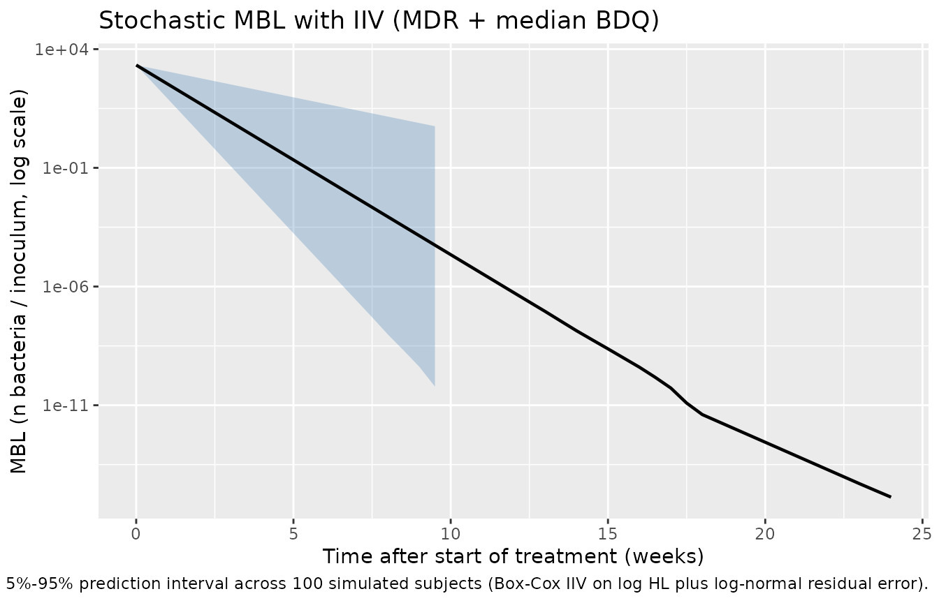
Cross-checks against the Svensson 2017 Results paragraph
Half-life shortening at observed bedaquiline exposure percentiles
Svensson 2017 (Results, ‘Covariate and PK effects’) reports that at
the 5th, 50th, and 95th percentile of observed bedaquiline
weekly-average concentrations at week 2, the typical half-life of
bacterial clearance is 32.8%, 51.6%, and 64.2% shorter than for a
typical placebo patient, respectively. Inverting the Emax formula
HL_i = HL_typ * EC50 / (EC50 + CAV) at
EC50 = 1.42 mg/L recovers the corresponding
CAV values:
hl_typ_weeks <- 0.81
ec50_bdq     <- 1.42

reported <- tibble::tibble(
  percentile        = c("5th",  "50th", "95th"),
  hl_shortening_pct = c(32.8,   51.6,   64.2)
) |>
  dplyr::mutate(
    bdq_factor   = 1 - hl_shortening_pct / 100,        # HL_i / HL_typ
    implied_cav  = ec50_bdq * (1 - bdq_factor) / bdq_factor,
    implied_hl   = hl_typ_weeks * bdq_factor
  )

knitr::kable(
  reported,
  digits  = c(NA, 1, 3, 3, 3),
  caption = "Implied bedaquiline CAV (mg/L) and individual MBL half-life (weeks) at the 5th/50th/95th observed-exposure percentiles per Svensson 2017 Results."
)| percentile | hl_shortening_pct | bdq_factor | implied_cav | implied_hl |
|---|---|---|---|---|
| 5th | 32.8 | 0.672 | 0.693 | 0.544 |
| 50th | 51.6 | 0.484 | 1.514 | 0.392 |
| 95th | 64.2 | 0.358 | 2.546 | 0.290 |
The implied median CAV of ~1.5 mg/L is the basis for the “median BDQ” scenario in the cohort table above. The 5th percentile CAV (~0.69 mg/L) is close to the “low BDQ” (0.75 mg/L) scenario, and the 95th percentile CAV (~2.55 mg/L) sits between the “median” and “high” (3.0 mg/L) scenarios.
Baseline-TTP effect on starting MBL_0
mbl0_typ_p     <- 2.14e3
ttp_ref_days   <- 6.8
e_ttp_mbl0     <- -3.69

ttp_grid <- tibble::tibble(
  TTP_MGIT_BASE = c(2.3, 4.0, 6.8, 10.0, 20.0, 42.0)
) |>
  dplyr::mutate(
    mbl0       = mbl0_typ_p * (TTP_MGIT_BASE / ttp_ref_days) ^ e_ttp_mbl0,
    rel_to_med = mbl0 / mbl0_typ_p
  )

knitr::kable(
  ttp_grid,
  digits  = c(1, 0, 2),
  caption = "Per-subject starting MBL_0 as a function of baseline mean TTP in MGIT (days). Reference 6.8 days is the cohort median (Svensson 2017 Table 1)."
)| TTP_MGIT_BASE | mbl0 | rel_to_med |
|---|---|---|
| 2.3 | 116841 | 54.60 |
| 4.0 | 15162 | 7.09 |
| 6.8 | 2140 | 1.00 |
| 10.0 | 516 | 0.24 |
| 20.0 | 40 | 0.02 |
| 42.0 | 3 | 0.00 |
A subject with TTP_MGIT_BASE = 2.3 days (cohort minimum,
fast-growing inoculum) has a starting MBL approximately 55x larger than
the typical (median-TTP) subject; conversely a subject with
TTP_MGIT_BASE = 42 days (cohort maximum, slow-growing
inoculum) has a starting MBL approximately 2.58572 n bacteria / inoculum
– essentially zero. This matches Svensson 2017 Discussion paragraph 3
(‘the estimated effect predicted a four times longer median TSCC in
patients with the lowest observed mTTP_0 compared with those with the
highest’).
Assumptions and deviations
- MBL is treated as the observable. The Svensson 2017 source does not observe MBL directly; it is the latent driver of MGIT TTP / probability-of-presence observations. The source’s full 3-component model (longitudinal MBL + per-sample lognormal IOV on the inoculum + logistic bacterial growth in the tube driving a Weibull-style time-to-positivity hazard with Bmax = 4.76e5 n bacteria, kg = 1.38e-6 (1/day per bacterium), hscale = 9.52e-5) is intentionally omitted. The extraction implements only Equation 1 of the source (the longitudinal MBL component) and folds the per-sample IOV_sputum variance (3.71 on log MBL) into the residual log-scale error on the latent state, so the simulated trajectories represent “what an idealised direct MBL measurement would see.” Reasoning: the probability-of-presence and tube-growth components are measurement-model artifacts of how the source authors inferred MBL from TTP data and have limited reuse value outside the original analysis, whereas the MBL decline (mono-exponential, with bedaquiline exposure and pre-XDR/XDR effects) is the biologically reusable PD component. Time-to-sputum-culture-conversion (TSCC) cannot be simulated from this extraction; users who need TSCC should reproduce the full Svensson 2017 model from the source’s supplementary code.
-
Bedaquiline weekly-average concentration is supplied as a
time-varying covariate (
CAV), not coupled to an upstream PK model. Svensson 2017 obtains individual CAV values as empirical-Bayes secondary metrics from the upstream Svensson 2016 (CPT PSP) population PK model for bedaquiline – shipped in nlmixr2lib asmodellib('Svensson_2016_bedaquiline'). Users who want a closed-loop PK-PD simulation can post-process a Svensson_2016_bedaquiline rxSolve into a 7-day rolling mean of the central-compartment concentration (in mg/L) and supply that as theCAVcolumn; this vignette uses constantCAVscenarios for illustration because (1) the flat scenarios match Table 3 / Figure 4 of the source (‘half median’, ‘median’, ‘double the median’ weekly average concentration), and (2) coupling the upstream PK adds many subject-level covariates (WT, ALB, AGE, RACE_BLACK) without changing the qualitative pattern. -
Constant
CAVover the simulation window. The source’s CAV is dynamic – it changes weekly because of the loading dose (week 1-2: 400 mg QD) versus maintenance (week 3+: 200 mg 3x/week) schedule and the slow accumulation of bedaquiline in tissues over weeks-to-months. This vignette holds CAV flat at each scenario’s representative value for clarity; a closed-loop coupling withmodellib('Svensson_2016_bedaquiline')would reproduce the time-varying envelope. The qualitative ordering of the scenarios (placebo > low > median > high; flatter trajectory for pre-XDR/XDR than MDR) is robust to this simplification. -
Box-Cox IIV form is taken from Petersson 2009 (reference 29
of the source). The NM-TRAN form
eta_BC = (exp(eta)^lambda - 1) / lambdais reproduced verbatim (matching howSchoemaker_2018_levetiracetam.Rencodes the same Petersson 2009 transformation); the source paper cites Petersson 2009 by reference but does not state the exact NM-TRAN code, and the online Supplementary Data containing the full NONMEM control stream was not on disk for this extraction. Variance 0.33 enters as the diagonal on the eta scale (pre-transform); shape lambda = 0.66 is held at its point-estimate value (no IIV on the shape itself, in line with the source which reports a single estimated shape per parameter). -
Pre-XDR and XDR strata are pooled
(
DIS_TB_XDR = 1reference category flagged in the canonical register). Svensson 2017 tested a separate effect for the missing-TB-type group and confirmed it did not differ significantly from MDR, so missing TB-type is assigned to the MDR /DIS_TB_XDR = 0reference group; this matches the source’s analytic decision (Results paragraph 4). -
The Svensson 2017 model has
emax_bdq = 1 FIX(maximum effect on HL = -100%). At very large CAV, the model predicts HL approaching 0 and unbounded killing rate, which is biologically implausible above the observed exposure range. Svensson 2017 explicitly cautions against extrapolation: ‘The maximal effect of bedaquiline could not be estimated due to the limited range of observed exposures. Extrapolation of the effect far outside the range of exposures included in the estimation of the relationship will be uncertain; this uncertainty may limit accuracy when using the model to simulate novel regimens with markedly higher bedaquiline doses’ (Discussion paragraph 7). Users simulating high-dose scenarios should treat the predicted half-life as a lower bound. -
The source’s online supplementary information (with the full
NONMEM model code) was not available on disk for this
extraction. The structural model is fully described in the main
paper’s Equations 1-3 and Table 2; the ambiguities the supplement would
have resolved (exact Box-Cox NM-TRAN form, the ordering of
multiplicative covariate factors on HL) have been resolved using the
Petersson 2009 cited form and the standard multiplicative ordering (IIV
factor first, then categorical covariate factor, then drug-effect
factor), with the chosen form documented in
model()comments and in this section. If the supplement is later obtained and disagrees with the chosen form, this extraction should be revisited.