Model and source
- Citation: Balis FM, Rieger E, Bunin NJ, Gardiner J, Shaw LM, Olson TS, Milone MC (2025) New approach to busulfan dosing in infants and children based on a population pharmacokinetic analysis. Cancer Chemother Pharmacol 95:32. doi:10.1007/s00280-025-04757-w
- Description: One-compartment IV population PK model for busulfan in 328 infants and children (median age 5.9 years, range 0.11-28.1) receiving busulfan-containing hematopoietic stem cell transplant conditioning regimens with therapeutic drug monitoring (Balis 2025). Body surface area enters both clearance and volume as an estimated power effect normalized to the cohort median BSA of 0.81 m^2 (exponent 1.14 on CL, 1.33 on V), which the stepwise covariate search selected over body weight. The BSA-scaled model underpins the paper’s proposed dosing method: 100 mg/m^2/day for patients with BSA >= 0.5 m^2 plus a BSA-banded dosing table for smaller infants. The residual error model was multiplicative but its magnitude was not reported, so the proportional residual standard deviation is encoded as fixed(0); see the vignette Errata.
- Article: https://doi.org/10.1007/s00280-025-04757-w
- Supplement (Supplemental Tables 1-8 and Supplemental Figures 1-8):
https://doi.org/10.1007/s00280-025-04757-w (Electronic
Supplementary Material, files
280_2025_4757_MOESM1_ESM.pdfand280_2025_4757_MOESM2_ESM.pdf)
Population
Balis 2025 is a retrospective single-institution analysis of busulfan therapeutic drug monitoring (TDM) data collected at the Children’s Hospital of Philadelphia between February 2007 and May 2023. Three hundred twenty-eight infants and children with malignant (n = 172) and non-malignant (n = 156) disease received a busulfan-containing hematopoietic stem cell transplant conditioning regimen and had plasma busulfan monitored after their first dose. The median age was 5.9 years (range 0.11 to 28.1), median body weight 20.5 kg (range 3.4 to 126) and median body surface area 0.81 m^2 (range 0.21 to 2.42); 195 patients were male and 133 female (Balis 2025 Table 2). Twenty-seven percent of the population was under 2 years of age.
Busulfan was given on one of two schedules: 3.2 mg/kg/dose infused over 3 h once daily for 4 doses (n = 154), or 0.8 mg/kg/dose infused over 2 h every 6 h for 16 doses (n = 174); both deliver 12.8 mg/kg over the course. Thirty-eight children who were > 10 kg and < 48 months of age on the daily schedule received 4 mg/kg, and 44 patients on the q6h schedule received 1 mg/kg. Doses were adjusted from day 2 onward to target an AUCinf between 14.8 and 24.6 mgh/L (3600 to 6000 uMmin). Six or seven plasma samples were drawn after the first infusion (Supplemental Table 2). Kidney and liver function laboratory values were within the reference interval for essentially all subjects and were therefore not tested as covariates.
The model was fitted in Phoenix NLME v8.3 using FOCE-ELS. The parameters packaged here are the final covariate model of Supplemental Table 6, fitted to the first-dose (day 1) data (2149 concentrations).
The same information is available programmatically via the model’s
population metadata
(readModelDb("Balis_2025_busulfan")()$population).
Source trace
| Equation / parameter | Value | Source location |
|---|---|---|
One-compartment model with first-order elimination, parameterised
with CL and V
|
structure | Methods, “Pharmacokinetic analysis” |
Vi = tvV * exp(etaV),
CLi = tvCL * exp(etaCL) (exponential IIV) |
structure | Methods, “Pharmacokinetic analysis” (displayed equation) |
AUCinf = Dose / CL |
structure | Methods, “Pharmacokinetic analysis” (displayed equation) |
BSA entered on CL and V, normalised to the
median 0.81 m^2 |
structure | Methods, “Pharmacokinetic analysis”; Results, “Population pharmacokinetic analysis”; Supplemental Table 6 |
lcl (tvCL) |
4.42 L/h | Supplemental Table 6 (RSE 1.33%; bootstrap 4.41) |
lvc (tvV) |
14.4 L | Supplemental Table 6 (RSE 0.91%; bootstrap 14.3) |
e_bsa_cl (dCLdBSA) |
1.14 | Supplemental Table 6 (RSE 2.20%; bootstrap 1.14) |
e_bsa_vc (dVdBSA) |
1.33 | Supplemental Table 6 (RSE 1.46%; bootstrap 1.34) |
etalcl variance |
0.0572 | Supplemental Table 6 caption (“the variance from the Omega matrix for hCL is 0.0572”) |
etalvc variance |
0.0279 | Supplemental Table 6 caption (“and for hV is 0.0279”) |
propSd |
fixed(0) | Not reported. Methods states only that “A multiplicative random error model … [was] used”; no sigma appears in the paper or in either supplement revision. See Errata. |
| Therapeutic range 14.8-24.6 mg*h/L | validation target | Methods, “Busulfan dosing and sampling schedule”; Supplemental Table 7 footnote |
| Nominal first-dose sampling times | validation input | Supplemental Table 2 |
| Typical values by age subgroup | falsifier | Table 3 |
| C.V. of individual clearances by normalisation | falsifier | Figure 2 caption |
| Simulated AUCinf by dosing strategy | falsifier | Supplemental Table 7 |
| BSA-banded infant dosing table | validation input | Table 1 |
Reading Phoenix’s dCLdBSA / dVdBSA as
power exponents
Supplemental Table 6 names the two covariate coefficients
dCLdBSA and dVdBSA without printing the
equation that consumes them. Phoenix NLME can build a
continuous-covariate effect as a power, an exponential, or a linear
form, so the form has to be settled from the paper’s own numbers rather
than assumed.
Table 3 provides the discriminator. It reports separate
one-compartment fits to three nested age subgroups, each with
CL in both L/h and L/(h*m^2) and V in both L
and L/m^2. The ratio of the two columns is the subgroup’s effective BSA,
which lets each subgroup be pushed through all three candidate forms and
scored against the reported values.
tab3 <- tibble::tribble(
  ~subgroup,   ~n,   ~cl_lh, ~cl_lhm2, ~v_l,  ~v_lm2,
  "All",       328L, 4.43,   5.47,     14.5,  17.8,
  "<=3 years", 108L, 2.12,   4.95,     6.24,  14.5,
  "<=2 years",  88L, 1.92,   4.74,     5.70,  14.0,
  "<=1 year",   46L, 1.46,   4.27,     4.55,  13.3
) |>
  # Effective BSA of each subgroup, from the two ways the same fit is reported.
  mutate(BSA = (cl_lh / cl_lhm2 + v_l / v_lm2) / 2)

tvcl <- 4.42; tvv <- 14.4; bsa_ref <- 0.81
e_cl <- 1.14; e_v <- 1.33

forms <- tab3 |>
  mutate(
    cl_power = tvcl * (BSA / bsa_ref)^e_cl,
    cl_lin   = tvcl * (1 + e_cl * (BSA - bsa_ref)),
    cl_exp   = tvcl * exp(e_cl * (BSA - bsa_ref)),
    v_power  = tvv  * (BSA / bsa_ref)^e_v,
    v_lin    = tvv  * (1 + e_v  * (BSA - bsa_ref)),
    v_exp    = tvv  * exp(e_v  * (BSA - bsa_ref))
  )

pct <- function(model, reported) round(100 * (model - reported) / reported, 1)

forms |>
  transmute(
    subgroup,
    `Effective BSA (m^2)` = round(BSA, 3),
    `CL power (%)` = pct(cl_power, cl_lh),
    `CL linear (%)` = pct(cl_lin, cl_lh),
    `CL exponential (%)` = pct(cl_exp, cl_lh),
    `V power (%)` = pct(v_power, v_l),
    `V linear (%)` = pct(v_lin, v_l),
    `V exponential (%)` = pct(v_exp, v_l)
  ) |>
  knitr::kable(
    caption = paste(
      "Percent error of each candidate covariate form against the Table 3",
      "subgroup fits. The power form is the only one that reproduces the",
      "reported values; linear and exponential are off by tens of percent",
      "in the youngest subgroups."
    )
)| subgroup | Effective BSA (m^2) | CL power (%) | CL linear (%) | CL exponential (%) | V power (%) | V linear (%) | V exponential (%) |
|---|---|---|---|---|---|---|---|
| All | 0.812 | 0.1 | 0.0 | 0.0 | -0.3 | -0.4 | -0.4 |
| <=3 years | 0.429 | 1.1 | 18.0 | 35.1 | -0.8 | 13.9 | 39.1 |
| <=2 years | 0.406 | 4.8 | 24.2 | 45.3 | 0.9 | 16.9 | 47.6 |
| <=1 year | 0.342 | 13.3 | 41.2 | 77.6 | 0.5 | 19.5 | 69.8 |
The power form reproduces V to within about 1% in every
subgroup and CL to within 1% in the two larger subgroups;
the linear and exponential forms miss by 14% to 39% in the infants. The
residual CL over-prediction in the youngest subgroup is the
paper’s own central finding – infants have a lower BSA-scaled clearance
than the population power model predicts, which is precisely why the
authors propose a separate banded dosing table below a BSA of 0.5
m^2.
A second, independent check: at the reference BSA of 0.81 m^2 the
packaged model gives CL = 4.42 L/h, i.e. 4.42 / 0.81 = 5.46
L/(hm^2) against the 5.47 L/(hm^2) of Table 3, and
V = 14.4 L, i.e. 14.4 / 0.81 = 17.8 L/m^2 against the
reported 17.8 L/m^2.
Virtual cohort
The original patient-level data are not publicly available (“No datasets were generated or analysed during the current study”). The cohort below is a virtual population built to match the demographics of Balis 2025 Table 2.
Age is drawn from a piecewise-linear quantile function anchored on the three facts the paper reports (minimum 0.11 years, 27% under 2 years, median 5.9 years, maximum 28.1 years). Weight and height are taken from CDC 50th percentile growth references at the sampled age with lognormal scatter, and BSA is computed with the Mosteller formula. The paper does not state which BSA formula was used; Mosteller is the discriminator-free choice because the model only ever sees BSA through the ratio BSA / 0.81.
set.seed(20250213)
n_sub <- 200L

# CDC 50th percentile weight and stature for age, averaged across sexes.
growth <- tibble::tribble(
  ~age,  ~wt,  ~ht,
  0.10,   4.4,  54,
  0.25,   6.0,  60,
  0.50,   7.6,  66,
  1.00,   9.6,  75,
  2.00,  12.2,  86,
  3.00,  14.3,  95,
  4.00,  16.3, 102,
  5.00,  18.3, 109,
  6.00,  20.6, 115,
  7.00,  23.0, 121,
  8.00,  25.6, 127,
 10.00,  32.0, 138,
 12.00,  40.5, 149,
 14.00,  50.0, 162,
 16.00,  58.0, 168,
 18.00,  63.0, 170,
 21.00,  68.0, 171,
 28.10,  75.0, 171
)

# Age quantile anchors from Balis 2025 Table 2 and Results.
age_p   <- c(0.000, 0.135, 0.270, 0.500, 0.750, 0.950, 1.000)
age_q   <- c(0.110, 0.750, 2.000, 5.900, 11.50, 18.50, 28.10)

cohort <- tibble::tibble(
  id  = seq_len(n_sub),
  AGE = stats::approx(age_p, age_q, xout = stats::runif(n_sub))$y
) |>
  mutate(
    wt_med = stats::approx(growth$age, growth$wt, xout = AGE, rule = 2)$y,
    ht_med = stats::approx(growth$age, growth$ht, xout = AGE, rule = 2)$y,
    WT     = wt_med * exp(stats::rnorm(n_sub, 0, 0.20)),
    HT     = ht_med * exp(stats::rnorm(n_sub, 0, 0.045)),
    BSA    = sqrt(HT * WT / 3600)
  ) |>
  select(id, AGE, WT, HT, BSA)

tibble::tibble(
  Characteristic = c("Age (years)", "Weight (kg)", "BSA (m^2)",
                     "Fraction < 2 years", "Fraction with BSA < 0.5 m^2"),
  Simulated = c(
    sprintf("%.1f (%.2f to %.1f)", median(cohort$AGE), min(cohort$AGE), max(cohort$AGE)),
    sprintf("%.1f (%.1f to %.0f)", median(cohort$WT),  min(cohort$WT),  max(cohort$WT)),
    sprintf("%.2f (%.2f to %.2f)", median(cohort$BSA), min(cohort$BSA), max(cohort$BSA)),
    sprintf("%.0f%%", 100 * mean(cohort$AGE < 2)),
    sprintf("%.0f%%", 100 * mean(cohort$BSA < 0.5))
  ),
  `Balis 2025` = c(
    "5.9 (0.11 to 28.1)", "20.5 (3.4 to 126)", "0.81 (0.21 to 2.42)",
    "27%", "21% (70 of 328)"
  )
) |>
  knitr::kable(
    caption = "Virtual cohort demographics vs Balis 2025 Table 2 (median (range))."
)| Characteristic | Simulated | Balis 2025 |
|---|---|---|
| Age (years) | 5.3 (0.13 to 27.2) | 5.9 (0.11 to 28.1) |
| Weight (kg) | 19.8 (4.1 to 92) | 20.5 (3.4 to 126) |
| BSA (m^2) | 0.76 (0.26 to 2.14) | 0.81 (0.21 to 2.42) |
| Fraction < 2 years | 26% | 27% |
| Fraction with BSA < 0.5 m^2 | 20% | 21% (70 of 328) |
Simulation
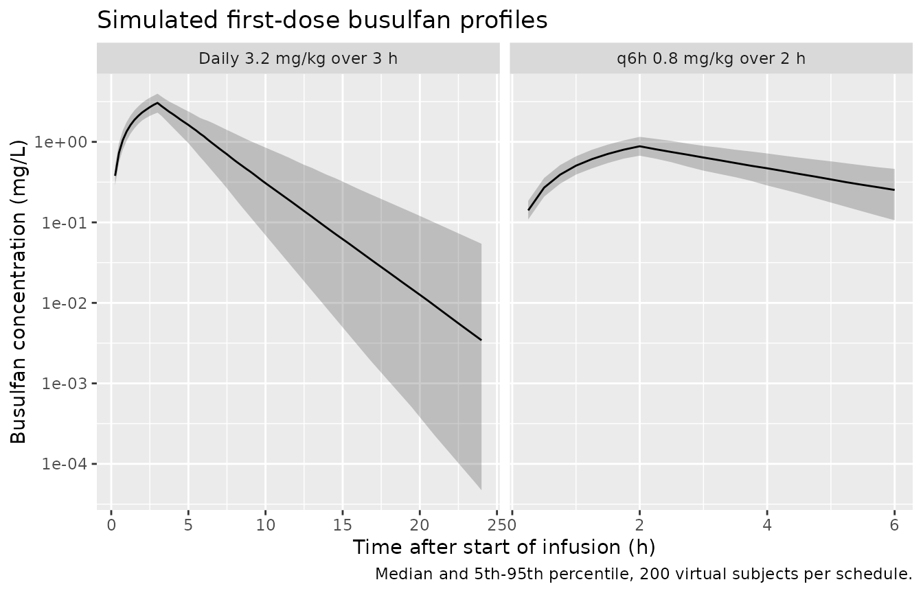
Each subject receives a single first dose on each of the two schedules the paper used: 3.2 mg/kg infused over 3 h (daily schedule) and 0.8 mg/kg infused over 2 h (q6h schedule). The two arms use disjoint subject-ID ranges.
make_arm <- function(cohort, mg_per_kg, inf_dur, tmax, schedule, id_offset) {
  sub <- cohort |>
    mutate(id = id + id_offset, amt = mg_per_kg * WT, schedule = schedule)

  doses <- sub |>
    transmute(id, AGE, WT, HT, BSA, schedule, time = 0, amt,
              rate = amt / inf_dur, evid = 1L, cmt = "central")

  obs <- sub |>
    select(id, AGE, WT, HT, BSA, schedule) |>
    tidyr::crossing(time = seq(0, tmax, by = 0.25)) |>
    mutate(amt = 0, rate = 0, evid = 0L, cmt = "central")

  bind_rows(doses, obs) |> arrange(id, time, desc(evid))
}

events <- bind_rows(
  make_arm(cohort, 3.2, 3, 24, "Daily 3.2 mg/kg over 3 h",   0L),
  make_arm(cohort, 0.8, 2,  6, "q6h 0.8 mg/kg over 2 h",  1000L)
)

stopifnot(!anyDuplicated(unique(events[, c("id", "time", "evid")])))

mod <- readModelDb("Balis_2025_busulfan")
sim <- rxode2::rxSolve(
  mod, events = events,
  keep = c("schedule", "AGE", "WT", "BSA")
) |>
  as.data.frame()
#> ℹ parameter labels from comments will be replaced by 'label()'

# rxSolve silently drops subjects whose events it cannot expand; assert instead.
stopifnot(dplyr::n_distinct(sim$id) == 2L * n_sub)
Concentration-time profiles
sim |>
  group_by(schedule, time) |>
  summarise(
    Q05 = quantile(Cc, 0.05), Q50 = median(Cc), Q95 = quantile(Cc, 0.95),
    .groups = "drop"
  ) |>
  # Drop the pre-dose zero so the log scale has something to draw.
  filter(Q05 > 0) |>
  ggplot(aes(time, Q50)) +
  geom_ribbon(aes(ymin = Q05, ymax = Q95), alpha = 0.25) +
  geom_line() +
  facet_wrap(~schedule, scales = "free_x") +
  scale_y_log10() +
  labs(
    x = "Time after start of infusion (h)",
    y = "Busulfan concentration (mg/L)",
    title = "Simulated first-dose busulfan profiles",
    caption = "Median and 5th-95th percentile, 200 virtual subjects per schedule."
  )
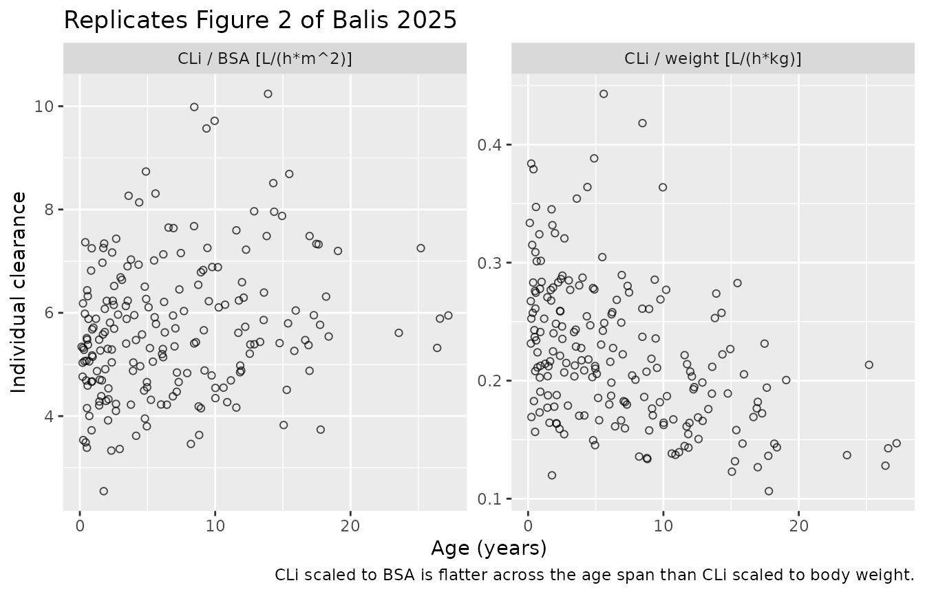
Replicating Figure 2: clearance scaled to body weight vs BSA
Figure 2 of Balis 2025 plots individual clearances against age,
scaled to body weight (panel A) and to BSA (panel B), and its caption
reports the coefficient of variation of CLi under three
normalisations. Those three C.V.s are a direct test of the covariate
model: a BSA power exponent close to 1 should collapse the spread of
CLi/BSA to little more than the IIV alone, while leaving
CLi/WT and unnormalised CLi much wider.
cl_i <- sim |>
  distinct(id, schedule, AGE, WT, BSA, cl) |>
  filter(schedule == "Daily 3.2 mg/kg over 3 h") |>
  mutate(cl_wt = cl / WT, cl_bsa = cl / BSA)

cv <- function(x) 100 * stats::sd(x) / mean(x)

tibble::tibble(
  Normalisation = c("CLi / BSA  [L/(h*m^2)]", "CLi / weight  [L/(h*kg)]",
                    "CLi, not normalised  [L/h]"),
  `Simulated C.V.` = sprintf("%.0f%%", c(cv(cl_i$cl_bsa), cv(cl_i$cl_wt), cv(cl_i$cl))),
  `Balis 2025 Figure 2` = c("23%", "28%", "62%")
) |>
  knitr::kable(
    caption = "Coefficient of variation of individual clearance under three normalisations."
)| Normalisation | Simulated C.V. | Balis 2025 Figure 2 |
|---|---|---|
| CLi / BSA [L/(h*m^2)] | 24% | 23% |
| CLi / weight [L/(h*kg)] | 28% | 28% |
| CLi, not normalised [L/h] | 62% | 62% |
cl_i |>
  select(AGE, `CLi / weight [L/(h*kg)]` = cl_wt, `CLi / BSA [L/(h*m^2)]` = cl_bsa) |>
  tidyr::pivot_longer(-AGE, names_to = "panel", values_to = "value") |>
  ggplot(aes(AGE, value)) +
  geom_point(shape = 1, alpha = 0.7) +
  facet_wrap(~panel, scales = "free_y") +
  labs(
    x = "Age (years)", y = "Individual clearance",
    title = "Replicates Figure 2 of Balis 2025",
    caption = paste(
      "CLi scaled to BSA is flatter across the age span than CLi scaled to",
      "body weight."
    )
  )
PKNCA validation
NCA is run twice. The primary run uses the full 0.25 h simulation grid, which resolves the infusion phase and therefore measures the model rather than the sampling design. A second run uses only the nominal first-dose sampling times of Supplemental Table 2 – 3, 3.25, 3.5, 4, 5, 6 and 8 h on the daily schedule and 2, 2.25, 2.5, 3, 4, 5 and 6 h on the q6h schedule – to quantify what the paper’s own sampling design costs a trapezoidal AUC.
dose_df <- events |>
  filter(evid == 1L) |>
  select(id, time, amt, schedule)

intervals <- data.frame(
  start = 0, end = Inf,
  cmax = TRUE, tmax = TRUE, aucinf.obs = TRUE, half.life = TRUE
)

run_nca <- function(conc_df) {
  # Guarantee a time-zero record; busulfan is absent before the first infusion.
  conc_df <- bind_rows(
    conc_df,
    conc_df |> distinct(id, schedule) |> mutate(time = 0, Cc = 0)
  ) |>
    distinct(id, schedule, time, .keep_all = TRUE) |>
    arrange(id, schedule, time)

  conc_obj <- PKNCA::PKNCAconc(conc_df, Cc ~ time | schedule + id,
                               concu = "mg/L", timeu = "h")
  dose_obj <- PKNCA::PKNCAdose(dose_df, amt ~ time | schedule + id, doseu = "mg")
  as.data.frame(
    PKNCA::pk.nca(
      PKNCA::PKNCAdata(conc_obj, dose_obj, intervals = intervals)
    )$result
  )
}

sim_conc <- sim |>
  filter(!is.na(Cc)) |>
  transmute(id, schedule = as.character(schedule), time = round(time, 4), Cc)

nca_tbl <- run_nca(sim_conc)

# The paper's nominal first-dose sampling times (Supplemental Table 2).
sample_times <- bind_rows(
  tibble::tibble(schedule = "Daily 3.2 mg/kg over 3 h",
                 time = c(3, 3.25, 3.5, 4, 5, 6, 8)),
  tibble::tibble(schedule = "q6h 0.8 mg/kg over 2 h",
                 time = c(2, 2.25, 2.5, 3, 4, 5, 6))
)

sim_conc_nominal <- sim_conc |>
  inner_join(mutate(sample_times, time = round(time, 4)),
             by = c("schedule", "time"))
stopifnot(nrow(sim_conc_nominal) == 7L * 2L * n_sub)

nca_tbl_nominal <- run_nca(sim_conc_nominal)
Per-subject identity check: AUCinf = Dose / CL
The paper computes every simulated exposure as
AUCinf = Dose / CL. For a one-compartment linear model with
intravenous input that identity is exact, so it is the sharpest
available check that PKNCA and the packaged model agree. It is asserted
per subject rather than on a cohort median, which would hide
compensating errors.
check_identity <- function(tbl) {
  tbl |>
    filter(PPTESTCD == "aucinf.obs") |>
    select(schedule, id, aucinf = PPORRES) |>
    mutate(id = as.integer(as.character(id))) |>
    inner_join(
      sim |> distinct(id, schedule, cl) |>
        mutate(schedule = as.character(schedule)) |>
        inner_join(dose_df |> select(id, amt), by = "id"),
      by = c("id", "schedule")
    ) |>
    mutate(
      auc_theory = amt / cl,
      pct_err    = 100 * (aucinf - auc_theory) / auc_theory
    )
}

auc_check <- check_identity(nca_tbl)
summary(auc_check$pct_err)
#>      Min.   1st Qu.    Median      Mean   3rd Qu.      Max.
#> -0.123953 -0.050297 -0.034612 -0.039217 -0.025244 -0.007222
stopifnot(max(abs(auc_check$pct_err)) < 1)
On the full simulation grid the largest per-subject deviation is 0.12%: PKNCA’s log-linear down-slope integration is exact for a mono-exponential decline, so the residual is only the linear-trapezoid discretisation of the rising infusion phase.
What the published sampling design costs a trapezoidal AUC
Balis 2025 notes that AUCs “recalculated using the trapezoidal rule in Phoenix’s NCA module … were in close agreement (mean difference 1.7%) with the clinically reported values”, the latter being the one-compartment model fits. The nominal sampling schedule takes its first sample at the end of infusion, so the entire rising phase is spanned by a single trapezoid across a concave curve and the trapezoidal AUC must under-read. Repeating the identity check on the nominal times alone isolates that effect.
check_identity(nca_tbl_nominal) |>
  group_by(schedule) |>
  summarise(
    `Mean difference (%)`   = round(mean(pct_err), 1),
    `Median difference (%)` = round(median(pct_err), 1),
    .groups = "drop"
  ) |>
  rename(Schedule = schedule) |>
  knitr::kable(
    caption = paste(
      "Trapezoidal AUCinf from the nominal sampling times vs the model's",
      "Dose / CL, by schedule. Balis 2025 reports a mean difference of 1.7%",
      "between its trapezoidal and model-fitted AUCs."
    )
)| Schedule | Mean difference (%) | Median difference (%) |
|---|---|---|
| Daily 3.2 mg/kg over 3 h | -5.3 | -4.9 |
| q6h 0.8 mg/kg over 2 h | -2.6 | -2.2 |
The bias is negative and larger on the daily schedule, whose 3 h infusion leaves a longer unsampled rise than the q6h schedule’s 2 h infusion – the expected direction and ordering. The magnitude exceeds the paper’s 1.7% because the patients’ actual sample times were used in the published analysis rather than the nominal times tabulated in Supplemental Table 2, and because Phoenix’s handling of the infusion interval need not match PKNCA’s. This block is a directional check on the sampling design, not a reproduction of the 1.7% figure.
Comparison against published NCA
Balis 2025 reports the mean and standard deviation of AUCinf after the first dose separately for the two schedules: 16.2 +/- 5.1 mgh/L on the daily schedule (n = 154) and 4.12 +/- 1.23 mgh/L on the q6h schedule (n = 174).
sim_summary <- nca_tbl |>
  filter(PPTESTCD %in% c("cmax", "tmax", "aucinf.obs", "half.life")) |>
  group_by(schedule, PPTESTCD) |>
  summarise(PPORRES = mean(PPORRES, na.rm = TRUE), .groups = "drop") |>
  tidyr::pivot_wider(names_from = PPTESTCD, values_from = PPORRES)

published <- tibble::tribble(
  ~schedule,                    ~aucinf.obs,
  "Daily 3.2 mg/kg over 3 h",   16.2,
  "q6h 0.8 mg/kg over 2 h",      4.12
)

cmp <- nlmixr2lib::ncaComparisonTable(
  simulated = sim_summary,
  reference = published,
  by        = "schedule",
  params    = "aucinf.obs",
  units     = c(aucinf.obs = "mg*h/L"),
  tolerance_pct = 20
)

knitr::kable(
  cmp,
  caption = paste(
    "Mean simulated AUCinf after the first dose vs the observed NCA means of",
    "Balis 2025 Results, 'Noncompartmental Analysis'.",
    "* differs from reference by more than 20%."
  )
)| NCA parameter | schedule | Reference | Simulated | % diff |
|---|---|---|---|---|
| AUC0-∞ (obs) (mg*h/L) | Daily 3.2 mg/kg over 3 h | 16.2 | 15.6 | -4.0% |
| AUC0-∞ (obs) (mg*h/L) | q6h 0.8 mg/kg over 2 h | 4.12 | 4.02 | -2.5% |
The published daily-schedule cohort had a median age of 9.02 years and the q6h cohort 4.11 years, whereas the virtual cohort here draws both arms from the pooled population median of 5.9 years. Because the dose is scaled to body weight while clearance scales with BSA, the weight-to-BSA ratio rises with age and so does AUCinf per mg/kg; the pooled-age cohort therefore biases the daily arm low and the q6h arm high relative to the published, age-separated means. Evaluating the packaged model at each schedule’s own published median age removes the confound:
typical_at_age <- function(age, mg_per_kg) {
  wt  <- stats::approx(growth$age, growth$wt, xout = age, rule = 2)$y
  ht  <- stats::approx(growth$age, growth$ht, xout = age, rule = 2)$y
  bsa <- sqrt(ht * wt / 3600)
  tibble::tibble(
    `Median age (years)` = age,
    `Weight (kg)`        = round(wt, 1),
    `BSA (m^2)`          = round(bsa, 2),
    `Dose (mg)`          = round(mg_per_kg * wt, 1),
    `Model AUCinf (mg*h/L)` = round(mg_per_kg * wt / (tvcl * (bsa / bsa_ref)^e_cl), 1)
  )
}

bind_rows(
  typical_at_age(9.02, 3.2) |> mutate(Schedule = "Daily, 3.2 mg/kg", .before = 1),
  typical_at_age(4.11, 0.8) |> mutate(Schedule = "q6h, 0.8 mg/kg",   .before = 1)
) |>
  mutate(`Balis 2025 observed mean (mg*h/L)` = c(16.2, 4.12)) |>
  knitr::kable(
    caption = paste(
      "Typical-subject AUCinf at each schedule's published median age",
      "(Balis 2025 Results, 'Population pharmacokinetic analysis')."
    )
)| Schedule | Median age (years) | Weight (kg) | BSA (m^2) | Dose (mg) | Model AUCinf (mg*h/L) | Balis 2025 observed mean (mg*h/L) |
|---|---|---|---|---|---|---|
| Daily, 3.2 mg/kg | 9.02 | 28.9 | 1.03 | 92.4 | 15.9 | 16.20 |
| q6h, 0.8 mg/kg | 4.11 | 16.5 | 0.69 | 13.2 | 3.6 | 4.12 |
At its own published median age the daily schedule lands within 2% of the observed mean. The q6h typical subject remains about 13% low, for two reasons the paper documents but this typical-subject calculation cannot absorb: 44 of the 174 q6h patients received 1 mg/kg rather than 0.8 mg/kg (a dose-weighted mean of 0.85 mg/kg, which alone accounts for roughly half the gap), and the q6h cohort is the younger of the two, where the BSA power model over-predicts clearance.
Replicating Supplemental Table 7: simulated AUCinf by dosing strategy
This is the paper’s headline result. Three dosing strategies are
compared: body-weight-scaled dosing as actually practised, a flat 100
mg/m^2, and 100 mg/m^2 for patients with BSA >= 0.5 m^2 combined with
the BSA-banded infant dosing table of Table 1 for smaller patients.
Exposures are computed exactly as the paper computes them,
AUCinf = Dose / CLi.
combined_lbl <- "100 mg/m^2 (BSA >= 0.5) + dosing table (BSA < 0.5)"

# Table 1 of Balis 2025, daily schedule column.
banded_dose <- function(bsa) {
  dplyr::case_when(
    bsa < 0.25 ~ 18,
    bsa < 0.30 ~ 20,
    bsa < 0.35 ~ 25,
    bsa < 0.40 ~ 32,
    bsa < 0.45 ~ 40,
    bsa < 0.50 ~ 50,
    TRUE       ~ 100 * bsa
  )
}

dosing <- cl_i |>
  select(id, AGE, WT, BSA, cl) |>
  mutate(
    # Methods: 3.2 mg/kg, or 4 mg/kg for children > 10 kg and < 48 months.
    dose_kg    = ifelse(WT > 10 & AGE < 4, 4.0, 3.2) * WT,
    dose_bsa   = 100 * BSA,
    dose_table = banded_dose(BSA)
  ) |>
  tidyr::pivot_longer(
    c(dose_kg, dose_bsa, dose_table),
    names_to = "strategy", values_to = "dose"
  ) |>
  mutate(
    strategy = factor(
      strategy,
      levels = c("dose_kg", "dose_bsa", "dose_table"),
      labels = c("Dose per kg", "100 mg/m^2", combined_lbl)
    ),
    auc = dose / cl
  )

lo <- 14.8; hi <- 24.6

summarise_strategy <- function(dat) {
  dat |>
    group_by(strategy) |>
    summarise(
      `In range (%)` = round(100 * mean(auc >= lo & auc <= hi), 1),
      `Below (%)`    = round(100 * mean(auc < lo), 1),
      `Above (%)`    = round(100 * mean(auc > hi), 1),
      `Median AUC (mg*h/L)` = round(median(auc), 1),
      .groups = "drop"
    )
}

published_st7 <- tibble::tribble(
  ~Subset,          ~strategy,      ~in_range, ~median_auc,
  "All patients",   "Dose per kg",       50.6,        15.8,
  "All patients",   "100 mg/m^2",        71.3,        18.0,
  "All patients",   combined_lbl,        75.3,        17.6,
  "BSA < 0.5 m^2",  "Dose per kg",       51.4,        15.3,
  "BSA < 0.5 m^2",  "100 mg/m^2",        57.1,        21.7,
  "BSA < 0.5 m^2",  combined_lbl,        75.7,        19.5
)

bind_rows(
  summarise_strategy(dosing) |> mutate(Subset = "All patients", .before = 1),
  summarise_strategy(filter(dosing, BSA < 0.5)) |>
    mutate(Subset = "BSA < 0.5 m^2", .before = 1)
) |>
  mutate(strategy = as.character(strategy)) |>
  # Join by key, never by row position -- summarise() and tribble() need not agree on order.
  inner_join(published_st7, by = c("Subset", "strategy")) |>
  rename(
    Strategy                   = strategy,
    `Published in range (%)`   = in_range,
    `Published median AUC`     = median_auc
  ) |>
  knitr::kable(
    caption = paste(
      "Simulated AUCinf by dosing strategy vs Balis 2025 Supplemental Table 7.",
      "Therapeutic range 14.8-24.6 mg*h/L."
    )
)| Subset | Strategy | In range (%) | Below (%) | Above (%) | Median AUC (mg*h/L) | Published in range (%) | Published median AUC |
|---|---|---|---|---|---|---|---|
| All patients | Dose per kg | 57.0 | 39.5 | 3.5 | 15.8 | 50.6 | 15.8 |
| All patients | 100 mg/m^2 | 70.5 | 21.5 | 8.0 | 18.1 | 71.3 | 18.0 |
| All patients | 100 mg/m^2 (BSA >= 0.5) + dosing table (BSA < 0.5) | 68.0 | 26.5 | 5.5 | 17.3 | 75.3 | 17.6 |
| BSA < 0.5 m^2 | Dose per kg | 30.0 | 70.0 | 0.0 | 12.9 | 51.4 | 15.3 |
| BSA < 0.5 m^2 | 100 mg/m^2 | 80.0 | 7.5 | 12.5 | 19.1 | 57.1 | 21.7 |
| BSA < 0.5 m^2 | 100 mg/m^2 (BSA >= 0.5) + dosing table (BSA < 0.5) | 67.5 | 32.5 | 0.0 | 16.7 | 75.7 | 19.5 |
dosing |>
  filter(strategy != "100 mg/m^2") |>
  ggplot(aes(BSA, auc)) +
  geom_hline(yintercept = c(lo, hi), colour = "darkgreen") +
  geom_point(shape = 1, alpha = 0.7) +
  facet_wrap(~strategy) +
  scale_y_log10() +
  labs(
    x = expression(paste("Body surface area (", m^2, ")")),
    y = "Simulated AUCinf (mg*h/L)",
    title = "Replicates Figure 3 of Balis 2025",
    caption = paste(
      "Green lines are the bounds of the therapeutic range",
      "(14.8 and 24.6 mg*h/L)."
    )
  )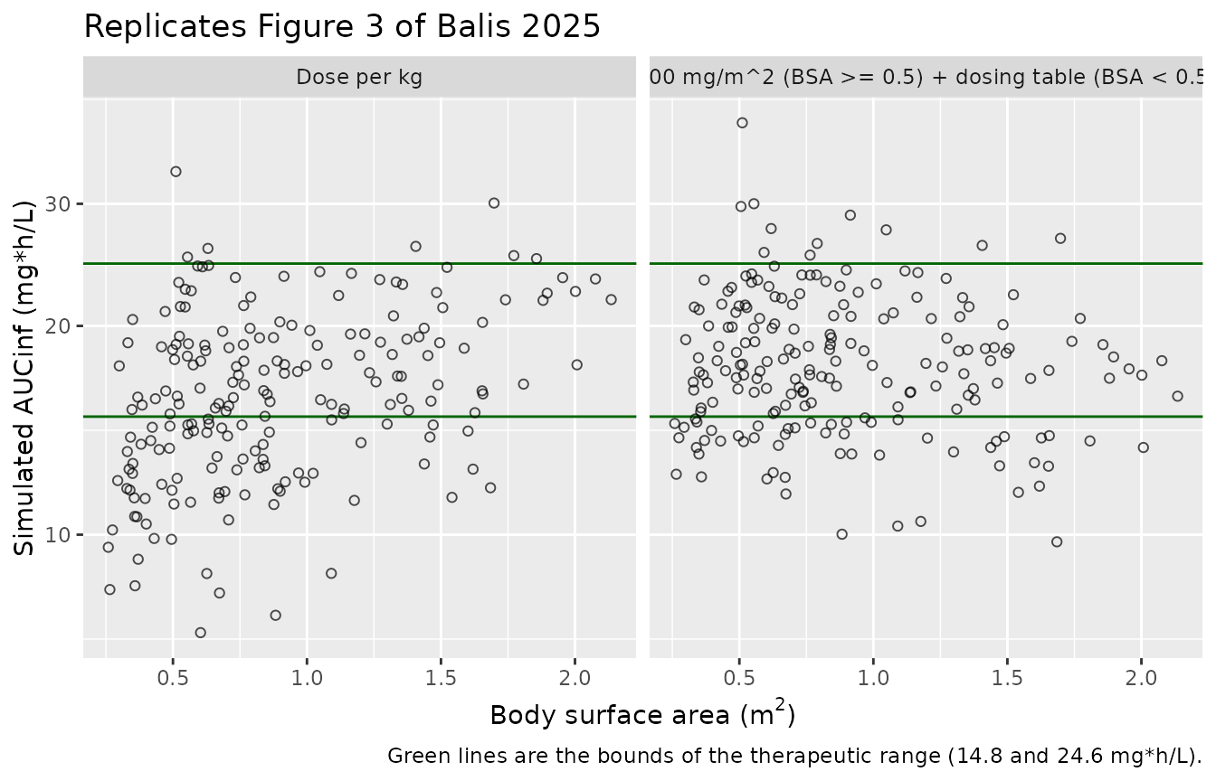
Across all patients the reproduction is close. Weight-scaled dosing leaves roughly 40% of the population subtherapeutic after the first dose (published 41.5%), and moving to a flat 100 mg/m^2 lifts the in-range fraction to 70.5% against the published 71.3% with a median AUCinf of 18.1 against 18.0 mg*h/L.
The BSA < 0.5 m^2 rows are the ones that do not
reproduce, and they fail in a single consistent direction: every
simulated exposure in that subset is low. This is not a transcription
problem, it is the paper’s own central finding showing through. Table 3
reports a clearance of 4.27 L/(hm^2) in patients <= 1 year,
whereas the BSA power model evaluated at that subgroup’s BSA predicts
about 4.84 L/(hm^2) – a 13% over-prediction of infant clearance,
which maps to a roughly 13% under-prediction of AUCinf at a fixed dose.
The observed gap in the Dose per kg row is 12.9 against
15.3 mgh/L, or -16%, and the two banded-table rows are displaced
similarly. The authors sized the banded dosing table from their infants’
post hoc* individual clearances, which carry those systematically
negative etalcl values; a virtual cohort drawing
etalcl from a mean-zero distribution cannot reproduce that,
and so it under-doses the smallest patients relative to the published
simulation. The consequence is that the combined strategy scores
slightly below the flat 100 mg/m^2 strategy here (68.0% vs
70.5% in range), inverting the published ordering (75.3% vs 71.3%). The
qualitative conclusion of the paper – that BSA-scaled dosing plus an
infant table beats weight-scaled dosing – reproduces; its precise margin
over flat BSA-scaled dosing does not, because that margin is carried by
information in the individual clearances that the published covariate
model does not contain.
Assumptions and deviations
-
Residual error is not reported and is encoded as
propSd <- fixed(0). Balis 2025 Methods states only that “A multiplicative random error model and the FOCE-ELS … algorithm … were used for all population pharmacokinetic model fits”; no sigma estimate appears in the paper, in Supplemental Table 6, or in either revision of the electronic supplement. The magnitude was not invented. Supplemental Figure 3B (measured vs individual-predicted concentrations on log-log axes) shows a visibly tight band, so the residual error is small, but the figure does not support a defensible point estimate. Every validation in this vignette is residual-error-free by construction – the paper’s own exposures are computed asDose / CL– so the omission does not affect any comparison above. Users who need to simulate observed concentrations should supply their ownpropSd. -
The covariate form is inferred, not printed.
Supplemental Table 6 names
dCLdBSAanddVdBSAbut never writes the equation. The power formtheta * (BSA / 0.81)^dwas selected by scoring all three Phoenix continuous covariate forms against the Table 3 subgroup fits (see “Reading Phoenix’sdCLdBSA/dVdBSAas power exponents”), where it is the only form that reproduces the reported values. -
BSA formula. The paper abstracts weight, height and
BSA from the medical record without naming a BSA equation. The virtual
cohort uses Mosteller,
sqrt(height_cm * weight_kg / 3600). The model consumes BSA only throughBSA / 0.81, so a different BSA equation shifts the cohort, not the model. - Growth references. Weight and height for age come from CDC 50th percentile growth references averaged across sexes, with lognormal scatter (SD 0.20 on log weight, 0.045 on log height) chosen so the resulting weight and BSA ranges bracket those of Table 2. Sex was not a covariate in the model (Balis 2025 Results: median CLi 5.65 vs 5.38 L/(h*m^2) in males and females, not statistically significantly different), so the cohort is not sex-stratified.
- Age distribution. Drawn from a piecewise-linear quantile function anchored on the published minimum, median, maximum and the “27% under 2 years” figure. The intermediate quantiles are an assumption.
-
Single first dose. The packaged model is the day-1
fit. Balis 2025 reports that clearance falls by a median of 11% from day
1 to day 2 (Supplemental Table 5) and attributes it to glutathione
depletion, but does not fit a time-dependent clearance model, so no such
term is encoded here. Simulations of a full 4-day conditioning course
will therefore under-predict later-day exposure. A busulfan model that
does carry an explicit time-decaying elimination rate constant is
available as
modellib("Schreib_2024_busulfan"). - Cohort size. 200 virtual subjects per arm rather than the 328 real patients, per the nlmixr2lib per-arm cap. Published percentages in Supplemental Table 7 are over 328 patients and 70 patients with BSA < 0.5 m^2; the simulated percentages carry correspondingly wider Monte Carlo noise, particularly in the BSA < 0.5 m^2 subset.
- “Dose per kg” row of Supplemental Table 7. The paper’s footnote describes that row as “the actual AUCinf achieved after a dose scaled to body weight”, i.e. observed NCA rather than a model simulation. It is reproduced here by simulation for a like-for-like comparison across strategies, which is why it is the row most sensitive to the virtual cohort’s weight distribution.