Model and source
- Citation: Hirai T, Kasai H, Naganuma M, Hagiwara N, Shiga T. Population pharmacokinetic analysis and dosage recommendations for digoxin in Japanese patients with atrial fibrillation and heart failure using real-world data. BMC Pharmacol Toxicol. 2022;23:14. doi:10.1186/s40360-022-00552-y.
- Description: One-compartment population PK model with first-order absorption for oral digoxin in 391 Japanese adults with atrial fibrillation and heart failure, fitted to routine steady-state trough serum concentrations (Hirai 2022). The absorption rate constant (1.0 1/h) and the apparent volume of distribution (6.0 L/kg, scaled linearly by body weight) were fixed from the literature; only the apparent oral clearance was estimated. CL/F scales as a power of Cockcroft-Gault creatinine clearance normalised to 60 mL/min (capped at 120 mL/min) and falls by a fractional 23.8% with concurrent amiodarone. Exponential between-subject variability on CL/F and a multiplicative (proportional) residual error. Companion Japanese digoxin trough model: Komatsu_2015_digoxin.
- Article: https://doi.org/10.1186/s40360-022-00552-y (open access)
mod <- readModelDb("Hirai_2022_digoxin")
ui <- rxode2::rxode(mod)
#> ℹ parameter labels from comments will be replaced by 'label()'
tv <- rxode2::zeroRe(mod)
#> ℹ parameter labels from comments will be replaced by 'label()'
Population
Hirai 2022 analysed 3465 trough serum digoxin concentrations from 391 consecutive Japanese adults with atrial fibrillation (AF) and heart failure (HF) who took oral digoxin at Tokyo Women’s Medical University Hospital between 2008 and 2016 (Methods; Table 1). All patients had ACC/AHA stage C or D HF. The cohort was elderly (67 +/- 14 years), light (57 +/- 15 kg) and 38% female, with a median Cockcroft-Gault creatinine clearance of 56.5 [40.7-75.6] mL/min and a mean LVEF of 39 +/- 14%. Most patients took 0.125 mg/day (73%); 13% took 0.25 mg/day and 10% took 0.0625 mg/day. 16% were on amiodarone, 8% on diltiazem and 6% on verapamil.
Concentrations drawn at least 6 h after the last dose and at least 5 days after the start of therapy were treated as steady-state troughs. Because only troughs were available, the authors fixed the absorption rate constant to 1.0 1/h and the apparent volume of distribution to 6.0 L/kg from the literature and estimated only the apparent oral clearance. The model was fitted in Phoenix NLME 8.1.
The same information is available programmatically via
ui$population.
Source trace
| Equation / parameter | Value | Source location |
|---|---|---|
| One-compartment, first-order absorption | n/a | Methods, Population pharmacokinetic model development; Results |
cl <- exp(lcl + etalcl) * (crcl_capped / 60)^e_crcl_cl * (1 + e_amio_cl * CONMED_AMIO) |
n/a | Results final model:
CL/F = 6.2 x (CLcr/60)^0.41 x (1 - 0.24 x [if amiodarone]);
exponential IIV per Methods CL/F = tv CL/F x exp(eta)
|
crcl_capped <- min(CRCL, 120) |
120 mL/min | Methods: CLcr above 120 mL/min replaced with 120 mL/min |
vc <- exp(lvc) * WT |
n/a | Results final model: Vd/F = 6.0 x Body weight
|
Cc <- 1000 * central / vc |
n/a | mg/L to ng/mL (Table 4 concentration units) |
lka |
fixed(log(1.0)) |
Table 3 ka (fixed) = 1.000 1/h |
lcl |
log(6.209) |
Table 3 CL/F = 6.209 L/h (RSE 2.83%) |
lvc |
fixed(log(6.0)) |
Table 3 Vd/F (fixed) = 6.000 L/kg |
e_crcl_cl |
0.409 | Table 3 CLCR on CL/F = 0.409 (RSE 9.49%) |
e_amio_cl |
-0.238 | Table 3 Amiodarone on CL/F = -0.238 (RSE 3.16%) |
etalcl |
0.344^2 = 0.118336 | Table 3 omega CL/F = 34.4% (RSE 2.9%) |
propSd |
0.366 | Table 3 Multiplicative = 36.6% (RSE 3.2%); Methods
Cobs = Cpred x (1 + eps)
|
The Results equation prints the thetas rounded to two digits (6.2, 0.41, 0.24); the model uses the three-decimal values of Table 3.
Validation
1. Typical clearance and steady-state trough
The paper’s clearance equation is evaluated directly and compared
with the model’s cl output, and the solved steady-state
trough is compared with the closed-form one-compartment
first-order-absorption trough
Ctrough = F D ka / (V (ka - k)) [exp(-k tau)/(1 - exp(-k tau)) - exp(-ka tau)/(1 - exp(-ka tau))].
Both sides use the same parameters, so the tolerances are numerical.
grid <- expand.grid(
  CRCL = c(30, 60, 90, 150),
  CONMED_AMIO = c(0, 1),
  dose = c(0.0625, 0.125, 0.25)
) |>
  mutate(id = row_number(), WT = 57)

ev_tv <- bind_rows(
  grid |> transmute(id, time = 0, amt = dose, ii = 24, ss = 1, evid = 1,
                    cmt = "depot", WT, CRCL, CONMED_AMIO),
  grid |> transmute(id, time = 24, amt = NA, ii = NA, ss = NA, evid = 0,
                    cmt = "central", WT, CRCL, CONMED_AMIO)
) |>
  arrange(id, time, desc(evid))

sim_tv <- rxode2::rxSolve(
  tv, events = ev_tv, returnType = "data.frame",
  rtol = 1e-10, atol = 1e-12, ssRtol = 1e-10, ssAtol = 1e-12, maxsteps = 1e6
) |>
  select(id, cl, vc, Cc) |>
  left_join(grid, by = "id")
#> ℹ omega/sigma items treated as zero: 'etalcl'
#> Warning: multi-subject simulation without without 'omega'

trough_closed <- function(dose, cl, v, ka = 1, tau = 24) {
  k <- cl / v
  1000 * dose * ka / (v * (ka - k)) *
    (exp(-k * tau) / (1 - exp(-k * tau)) - exp(-ka * tau) / (1 - exp(-ka * tau)))
}

chk_tv <- sim_tv |>
  mutate(
    cl_paper = 6.209 * (pmin(CRCL, 120) / 60)^0.409 * (1 - 0.238 * CONMED_AMIO),
    trough_closed = trough_closed(dose, cl_paper, 6 * WT)
  )

stopifnot(
  nrow(chk_tv) == nrow(grid),
  max(abs(chk_tv$cl / chk_tv$cl_paper - 1)) < 1e-12,
  # CRCL cap: 150 mL/min gives the same clearance as 120 mL/min.
  all(abs(chk_tv$cl[chk_tv$CRCL == 150] -
            6.209 * 2^0.409 * (1 - 0.238 * chk_tv$CONMED_AMIO[chk_tv$CRCL == 150])) < 1e-12),
  max(abs(chk_tv$Cc / chk_tv$trough_closed - 1)) < 1e-6
)

chk_tv |>
  filter(CRCL != 150) |>
  transmute(
    `Daily dose (mg)` = dose, `CLcr (mL/min)` = CRCL,
    Amiodarone = ifelse(CONMED_AMIO == 1, "yes", "no"),
    `CL/F (L/h)` = signif(cl, 4),
    `Typical trough (ng/mL)` = signif(Cc, 3)
  ) |>
knitr::kable(caption = "Typical-value clearance and steady-state trough (57 kg).")| Daily dose (mg) | CLcr (mL/min) | Amiodarone | CL/F (L/h) | Typical trough (ng/mL) |
|---|---|---|---|---|
| 0.0625 | 30 | no | 4.676 | 0.477 |
| 0.0625 | 60 | no | 6.209 | 0.341 |
| 0.0625 | 90 | no | 7.329 | 0.278 |
| 0.0625 | 30 | yes | 3.563 | 0.650 |
| 0.0625 | 60 | yes | 4.731 | 0.471 |
| 0.0625 | 90 | yes | 5.585 | 0.387 |
| 0.1250 | 30 | no | 4.676 | 0.954 |
| 0.1250 | 60 | no | 6.209 | 0.682 |
| 0.1250 | 90 | no | 7.329 | 0.555 |
| 0.1250 | 30 | yes | 3.563 | 1.300 |
| 0.1250 | 60 | yes | 4.731 | 0.941 |
| 0.1250 | 90 | yes | 5.585 | 0.774 |
| 0.2500 | 30 | no | 4.676 | 1.910 |
| 0.2500 | 60 | no | 6.209 | 1.360 |
| 0.2500 | 90 | no | 7.329 | 1.110 |
| 0.2500 | 30 | yes | 3.563 | 2.600 |
| 0.2500 | 60 | yes | 4.731 | 1.880 |
| 0.2500 | 90 | yes | 5.585 | 1.550 |
2. Reproduction of Table 4 (probability of a toxic-range trough)
Hirai 2022 Table 4 gives, from a 1000-subject Monte Carlo simulation of the final model, the probability that a steady-state trough is at least 0.9 ng/mL or 1.2 ng/mL, for three daily doses, three CLcr values and with or without amiodarone. The paper does not state the body weight used; the cohort mean of 57 kg (Table 1) is assumed. Body weight only moves the trough through the fixed volume, so it has a small effect.
Instead of a random cohort, the between-subject distribution of CL/F
is integrated with 200 stratified quantiles of etalcl per
cell, supplied through params, and the multiplicative
residual error Cobs = Cpred x (1 + eps) is integrated
analytically:
P(Cobs >= c) = 1 - Phi((c / Cpred - 1) / propSd). The
result is the exact model probability to within quadrature error, and
does not depend on the random-number stream.
omega_cl <- ui$omega["etalcl", "etalcl"]
prop_sd <- ui$theta[["propSd"]]
nq <- 200

table4 <- tibble::tribble(
  ~dose,  ~CRCL, ~CONMED_AMIO, ~pub_09, ~pub_12,
  0.25,   90, 0, 61.9, 43.0,
  0.25,   60, 0, 72.7, 55.7,
  0.25,   30, 0, 86.9, 76.3,
  0.125,  90, 0, 18.7,  7.0,
  0.125,  60, 0, 28.1, 12.4,
  0.125,  30, 0, 51.3, 31.1,
  0.0625, 90, 0,  0.9,  0.0,
  0.0625, 60, 0,  1.8,  0.5,
  0.0625, 30, 0, 11.2,  3.1,
  0.25,   90, 1, 79.0, 65.7,
  0.25,   60, 1, 86.4, 74.5,
  0.25,   30, 1, 95.0, 88.1,
  0.125,  90, 1, 37.1, 19.0,
  0.125,  60, 1, 51.6, 31.5,
  0.125,  30, 1, 71.4, 54.4,
  0.0625, 90, 1,  3.7,  0.7,
  0.0625, 60, 1,  8.2,  1.7,
  0.0625, 30, 1, 24.3, 10.6
)

subj4 <- table4 |>
  mutate(cell = row_number()) |>
  tidyr::crossing(q = seq_len(nq)) |>
  mutate(
    id = row_number(),
    WT = 57,
    etalcl = sqrt(omega_cl) * qnorm((q - 0.5) / nq)
  )

ev4 <- bind_rows(
  subj4 |> transmute(id, time = 0, amt = dose, ii = 24, ss = 1, evid = 1,
                     cmt = "depot", WT, CRCL, CONMED_AMIO),
  subj4 |> transmute(id, time = 24, amt = NA, ii = NA, ss = NA, evid = 0,
                     cmt = "central", WT, CRCL, CONMED_AMIO)
) |>
  arrange(id, time, desc(evid))

# The etas are supplied through `params`, so no omega sampling is wanted:
# the typical-value model is solved and rxode2 would otherwise warn that a
# multi-subject simulation carries no omega.
sim4 <- suppressWarnings(rxode2::rxSolve(
  tv, events = ev4, params = subj4 |> select(id, etalcl),
  returnType = "data.frame", maxsteps = 1e6
)) |>
  select(id, cl, Cc) |>
  left_join(subj4 |> select(id, cell, dose, CRCL, CONMED_AMIO, etalcl), by = "id")

# Guard: every subject's clearance must carry its own supplied eta. A harness
# that silently drops `params` etas would solve everyone at the typical value.
cl_expected <- with(sim4, 6.209 * (pmin(CRCL, 120) / 60)^0.409 *
                      (1 - 0.238 * CONMED_AMIO) * exp(etalcl))
stopifnot(nrow(sim4) == nrow(subj4), max(abs(sim4$cl / cl_expected - 1)) < 1e-8)

pta <- sim4 |>
  group_by(cell, dose, CRCL, CONMED_AMIO) |>
  summarise(
    n = n(),
    sim_09 = 100 * mean(1 - pnorm((0.9 / Cc - 1) / prop_sd)),
    sim_12 = 100 * mean(1 - pnorm((1.2 / Cc - 1) / prop_sd)),
    nores_09 = 100 * mean(Cc >= 0.9),
    nores_12 = 100 * mean(Cc >= 1.2),
    .groups = "drop"
  ) |>
  left_join(table4, by = c("dose", "CRCL", "CONMED_AMIO")) |>
  mutate(diff_09 = sim_09 - pub_09, diff_12 = sim_12 - pub_12)

diffs <- c(pta$diff_09, pta$diff_12)
diffs_nores <- c(pta$nores_09 - pta$pub_09, pta$nores_12 - pta$pub_12)
stopifnot(
  nrow(pta) == 18L,
  all(pta$n == nq),
  # The published values carry Monte Carlo error from 1000 draws (binomial
  # SE up to 1.6 percentage points at p = 0.5), and the simulation weight is
  # not stated. Measured: median |diff| 0.5, maximum 1.9 points. A
  # mis-transcribed clearance, exponent or amiodarone factor moves the
  # mid-range cells by 5-20 points.
  median(abs(diffs)) < 1.5,
  max(abs(diffs)) < 4,
  # Without residual error the reproduction is clearly worse.
  max(abs(diffs_nores)) > 3 * max(abs(diffs))
)

pta |>
  transmute(
    `Dose (mg/day)` = dose, `CLcr (mL/min)` = CRCL,
    Amiodarone = ifelse(CONMED_AMIO == 1, "yes", "no"),
    `>= 0.9 model` = round(sim_09, 1), `>= 0.9 paper` = pub_09,
    `>= 1.2 model` = round(sim_12, 1), `>= 1.2 paper` = pub_12
  ) |>
knitr::kable(caption = "Replicates Table 4 of Hirai 2022: percentage of steady-state troughs at or above 0.9 and 1.2 ng/mL.")| Dose (mg/day) | CLcr (mL/min) | Amiodarone | >= 0.9 model | >= 0.9 paper | >= 1.2 model | >= 1.2 paper |
|---|---|---|---|---|---|---|
| 0.2500 | 90 | no | 60.8 | 61.9 | 41.5 | 43.0 |
| 0.2500 | 60 | no | 73.0 | 72.7 | 55.7 | 55.7 |
| 0.2500 | 30 | no | 87.2 | 86.9 | 76.2 | 76.3 |
| 0.1250 | 90 | no | 16.8 | 18.7 | 6.3 | 7.0 |
| 0.1250 | 60 | no | 28.0 | 28.1 | 12.7 | 12.4 |
| 0.1250 | 30 | no | 51.2 | 51.3 | 30.8 | 31.1 |
| 0.0625 | 90 | no | 0.9 | 0.9 | 0.1 | 0.0 |
| 0.0625 | 60 | no | 2.4 | 1.8 | 0.4 | 0.5 |
| 0.0625 | 30 | no | 9.5 | 11.2 | 2.7 | 3.1 |
| 0.2500 | 90 | yes | 79.4 | 79.0 | 64.2 | 65.7 |
| 0.2500 | 60 | yes | 86.8 | 86.4 | 75.5 | 74.5 |
| 0.2500 | 30 | yes | 94.0 | 95.0 | 88.3 | 88.1 |
| 0.1250 | 90 | yes | 36.3 | 37.1 | 18.5 | 19.0 |
| 0.1250 | 60 | yes | 50.3 | 51.6 | 29.9 | 31.5 |
| 0.1250 | 30 | yes | 71.7 | 71.4 | 53.0 | 54.4 |
| 0.0625 | 90 | yes | 4.2 | 3.7 | 0.9 | 0.7 |
| 0.0625 | 60 | yes | 9.0 | 8.2 | 2.6 | 1.7 |
| 0.0625 | 30 | yes | 24.3 | 24.3 | 9.9 | 10.6 |
The packaged model reproduces every cell of Table 4 to within 1.9
percentage points (median absolute difference 0.47). The agreement also
supports two readings that the paper leaves implicit: the Monte Carlo
simulation included the multiplicative residual error (without it the
predicted probabilities differ from Table 4 by up to 12 points), and the
residual error enters as a normal eps on the (1 + eps)
scale.
3. Distribution of simulated troughs (Figure 2)
Figure 2 of Hirai 2022 shows violin plots of the predicted troughs by
dose and CLcr, without and with amiodarone. A stochastic cohort of 100
subjects per cell is simulated here with residual error
(sim), the observable the Monte Carlo simulation
summarised.
rxode2::rxSetSeed(20220214)
cells <- table4 |> select(dose, CRCL, CONMED_AMIO) |> mutate(cell = row_number())
subj2 <- cells |>
  tidyr::crossing(k = seq_len(100)) |>
  mutate(id = row_number(), WT = 57)

ev2 <- bind_rows(
  subj2 |> transmute(id, time = 0, amt = dose, ii = 24, ss = 1, evid = 1,
                     cmt = "depot", WT, CRCL, CONMED_AMIO),
  subj2 |> transmute(id, time = 24, amt = NA, ii = NA, ss = NA, evid = 0,
                     cmt = "central", WT, CRCL, CONMED_AMIO)
) |>
  arrange(id, time, desc(evid))

sim2 <- rxode2::rxSolve(mod, events = ev2, returnType = "data.frame",
                        maxsteps = 1e6) |>
  select(id, Cc, sim) |>
  left_join(subj2 |> select(id, dose, CRCL, CONMED_AMIO), by = "id")
#> ℹ parameter labels from comments will be replaced by 'label()'

stopifnot(nrow(sim2) == nrow(subj2), all(is.finite(sim2$sim)))

ggplot(sim2 |> mutate(
  Dose = factor(paste(dose, "mg"), levels = paste(c(0.25, 0.125, 0.0625), "mg")),
  CLcr = factor(paste(CRCL, "mL/min"), levels = paste(c(90, 60, 30), "mL/min")),
  Amiodarone = ifelse(CONMED_AMIO == 1, "With amiodarone", "Without amiodarone")
), aes(CLcr, pmax(sim, 0.01), fill = Dose)) +
  geom_violin(position = position_dodge(0.9), draw_quantiles = c(0.25, 0.5, 0.75),
              scale = "width") +
  geom_hline(yintercept = c(0.9, 1.2), linetype = "dashed") +
  facet_wrap(~Amiodarone) +
  scale_y_log10() +
  labs(x = "Creatinine clearance", y = "Trough serum digoxin (ng/mL)",
       caption = "Replicates Figure 2 of Hirai 2022 (57 kg; residual error included).")
#> Warning: The `draw_quantiles` argument of `geom_violin()` is deprecated as of ggplot2
#> 4.0.0.
#> ℹ Please use the `quantiles.linetype` argument instead.
#> This warning is displayed once per session.
#> Call `lifecycle::last_lifecycle_warnings()` to see where this warning was
#> generated.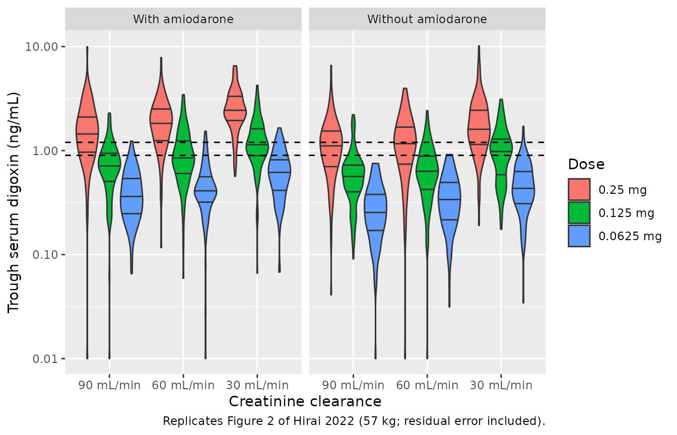
4. Steady-state NCA with PKNCA
The paper reports no NCA. PKNCA is used here to check that the
model’s steady-state dosing-interval exposure matches its clearance: at
steady state AUC0-24 = F x Dose / (CL/F), and
Cavg = AUC0-24 / 24. A stochastic cohort of 100 subjects
per CLcr / amiodarone group is dosed 0.125 mg once daily to steady state
and sampled every 0.5 h over one interval.
rxode2::rxSetSeed(20220215)
grp <- expand.grid(CRCL = c(30, 60, 90), CONMED_AMIO = c(0, 1)) |>
  mutate(treatment = paste0("CLcr ", CRCL, ifelse(CONMED_AMIO == 1, " + amiodarone", "")))
subj_nca <- grp |>
  tidyr::crossing(k = seq_len(100)) |>
  mutate(id = row_number(), WT = pmin(pmax(rnorm(n(), 57, 15), 35), 100))

ev_nca <- bind_rows(
  subj_nca |> transmute(id, time = 0, amt = 0.125, ii = 24, ss = 1, evid = 1,
                        cmt = "depot", WT, CRCL, CONMED_AMIO),
  subj_nca |> tidyr::crossing(time = seq(0, 24, by = 0.5)) |>
    transmute(id, time, amt = NA, ii = NA, ss = NA, evid = 0,
              cmt = "central", WT, CRCL, CONMED_AMIO)
) |>
  arrange(id, time, desc(evid))

sim_nca <- rxode2::rxSolve(mod, events = ev_nca, returnType = "data.frame",
                           maxsteps = 1e6) |>
  select(id, time, Cc, cl) |>
  left_join(subj_nca |> select(id, treatment), by = "id")

conc <- sim_nca |>
  filter(!is.na(Cc)) |>
  select(id, time, Cc, treatment)
dose_df <- subj_nca |> transmute(id, time = 0, amt = 0.125, treatment)

pk_conc <- PKNCA::PKNCAconc(conc, Cc ~ time | treatment + id)
pk_dose <- PKNCA::PKNCAdose(dose_df, amt ~ time | treatment + id)
intervals <- data.frame(start = 0, end = 24, auclast = TRUE, cmax = TRUE,
                        tmax = TRUE, cmin = TRUE, cav = TRUE)
nca <- PKNCA::pk.nca(PKNCA::PKNCAdata(pk_conc, pk_dose, intervals = intervals))
nca_res <- as.data.frame(nca$result)

auc_chk <- nca_res |>
  filter(PPTESTCD == "auclast") |>
  select(id, treatment, auc = PPORRES) |>
  left_join(sim_nca |> distinct(id, cl), by = "id") |>
  mutate(auc_theory = 1000 * 0.125 / cl, rel = auc / auc_theory - 1)

stopifnot(
  nrow(auc_chk) == nrow(subj_nca),
  # Same drawn parameters on both sides; the only difference is trapezoidal
  # error over a 0.5 h grid (measured below 0.2%).
  max(abs(auc_chk$rel)) < 0.01
)

summary(nca)
#>  start end            treatment   N     auclast         cmax         cmin
#>      0  24              CLcr 30 100 27.1 [31.1]  1.28 [27.1] 0.955 [37.5]
#>      0  24 CLcr 30 + amiodarone 100 34.3 [37.8]  1.58 [34.0]  1.25 [43.5]
#>      0  24              CLcr 60 100 19.6 [35.2] 0.980 [28.6] 0.637 [47.6]
#>      0  24 CLcr 60 + amiodarone 100 27.7 [35.1]  1.30 [31.2] 0.984 [41.4]
#>      0  24              CLcr 90 100 16.8 [37.8] 0.871 [29.9] 0.517 [53.0]
#>      0  24 CLcr 90 + amiodarone 100 22.0 [33.8]  1.07 [28.3] 0.740 [43.2]
#>               tmax          cav
#>  3.00 [3.00, 3.00]  1.13 [31.1]
#>  3.00 [3.00, 3.00]  1.43 [37.8]
#>  3.00 [2.50, 3.00] 0.817 [35.2]
#>  3.00 [3.00, 3.00]  1.15 [35.1]
#>  3.00 [2.50, 3.00] 0.701 [37.8]
#>  3.00 [3.00, 3.00] 0.916 [33.8]
#>
#> Caption: auclast, cmax, cmin, cav: geometric mean and geometric coefficient of variation; tmax: median and range; N: number of subjects
Assumptions and deviations
-
Omega scale. Table 3 prints
omega CL/F = 34.4%. The model takes this as the SD of the exponential eta (variance0.344^2 = 0.118). The alternative CV reading,log(1 + 0.344^2) = 0.112, differs by 5.6% in variance. When Table 4 is re-derived with the method above, the SD reading reproduces it slightly better (RMSE 0.84 vs 0.94 percentage points at 57 kg), which is consistent with but does not prove the choice. - Simulation body weight. Table 4 and Figure 2 do not state the weight used in the Monte Carlo simulation; the cohort mean of 57 kg (Table 1) is used. Weights of 50 and 65 kg reproduce Table 4 less well (RMSE 1.8 and 1.0 points).
- Trough time. Troughs are evaluated 24 h after a once-daily dose at steady state. The paper’s troughs were drawn at least 6 h after the last dose, so real sampling times varied.
-
CLcr cap. The Methods cap of 120 mL/min is applied
inside
model(), so users supply the uncapped Cockcroft-Gault value inCRCL. -
Bioavailability. Only CL/F and Vd/F are
identifiable; there is no
Fin the model and the dose is the administered oral amount. - Amiodarone dose. The amiodarone effect is a single fractional decrease in CL/F; the paper did not model amiodarone dose.
- Errata. A EuropePMC search on 2026-09-30 found no correction notice for this article.