Methylprednisolone (Cleary 2026)
Source:vignettes/articles/Cleary_2026_methylprednisolone.Rmd
Cleary_2026_methylprednisolone.RmdModel and source
- Citation: Cleary H, Fotaki N, Persoons T, D’Arcy DM. Using PBPK to Simulate Target Biopredictive Dissolution Profiles for Long-Acting Injectables - Where to Begin With Critical Bioavailability Attributes? CPT Pharmacometrics Syst Pharmacol. 2026;15(3):e70212. doi:10.1002/psp4.70212. Disposition parameters are from Table 1; the peripheral-to-central rate constant K21 is not printed and was back-solved from the simulated concentration at 0.18 h in Supplementary Table S1.
- Description: PBPK (GastroPlus 8.3.3) long-acting intramuscular methylprednisolone acetate paper, compartmental disposition layer. Two-compartment intravenous methylprednisolone model in a 70 kg adult with body-weight-proportional central volume and clearance, fitted with the GastroPlus PKPlus module to published mean plasma concentrations after an 80 mg intravenous bolus of methylprednisolone sodium succinate. The paper’s mechanistic intramuscular depot (particle dissolution and injection-site absorption) and its simulated in vivo dissolution profiles are not included (see the vignette). Deterministic typical-value model with no between-subject or residual variability.
- Article: https://doi.org/10.1002/psp4.70212 (open access, PMC12916861)
Cleary and colleagues used GastroPlus 8.3.3 to model the long-acting intramuscular (IM) suspension of methylprednisolone acetate (80 mg/mL, Depo-Medrol and its generics). Their aim was to find which critical bioavailability attributes (particle size, solubility, diffusion layer thickness, diffusion coefficient and depot volume) reproduce the observed plasma profile, and to turn the simulated in vivo dissolution of the best models (A to D, Figure 4) into target profiles for biopredictive in vitro dissolution testing.
The systemic disposition of methylprednisolone is not a whole-body PBPK model. In step 1 of the workflow the authors fitted 1-, 2- and 3-compartment models with the GastroPlus PKPlus module to a published mean profile after an 80 mg intravenous (IV) bolus of methylprednisolone sodium succinate (in vivo dataset A), selected the 2-compartment model and carried its parameters into every IM simulation (Table 1).
What this model contains
This model is that IV disposition model: central volume 0.84106 L/kg, clearance 0.46751 L/h/kg and K12 45.107 1/h (Table 1), for the 70 kg GastroPlus default body weight, with volume and clearance proportional to body weight as GastroPlus scales per-kg compartmental parameters.
Table 1 does not print the fourth parameter, K21. It was back-solved from Supplementary Table S1, which gives the simulated concentration at 0.18 h after the 80 mg bolus as 842 ng/mL: with the three printed parameters, only K21 = 89.14 1/h reproduces it (88.98 to 89.31 1/h across the rounding interval of 842). The section “Checks against the paper” tests that value against quantities that were not used to derive it.
The IM layer is not included. GastroPlus’s IM model dissolves the particles in a depot (a Johnson-type dissolution driven by particle size, solubility, diffusion coefficient and diffusion layer thickness) and absorbs the dissolved drug through the injection-site tissue. The paper prints the drug-side inputs (Tables 1 and 2, Supplementary Table S4), but the depot geometry, the local tissue volume, blood and lymph flows and the equations that connect them are built into the platform and are not reported. The simulated dissolution profiles of Figure 4 are outputs of that platform model, not fitted release functions, so they cannot be reproduced or re-encoded either.
Population
No individual data were fitted. The disposition model was fitted to one digitised mean profile after an 80 mg IV bolus of methylprednisolone sodium succinate (Al-Habet and Rogers 1989; 18 time points to 10 h, Supplementary S2 Table S2_1). The paper does not report the size or the demographics of that study. The simulations use the GastroPlus default body weight of 70 kg (Table 1).
Source trace
| Quantity | Value | Source |
|---|---|---|
| Structure | 2-compartment, IV bolus into central | Methods step 1; Results step 1 (‘A 2-compartmental model was considered adequate’); Table 1 ‘PK model’ |
lvc |
log(0.84106) L/kg | Table 1 ‘Volume of distribution (Vd)’ |
lk12 |
log(45.107) 1/h | Table 1 ‘K12’ |
lk21 |
log(89.14) 1/h | Back-solved from Supplementary Table S1, simulated ‘Cmax’ 842 ng/mL at ‘Tmax’ 0.18 h |
lcl |
log(0.46751) L/h/kg | Table 1 ‘Clearance (Cl)’ |
| Reference weight | 70 kg | Table 1 ‘Body weight’ (GastroPlus default) |
| Dose | 80 mg IV bolus | Methods step 1; Supplementary Figure S1 title |
| Observed profile | 18 mean concentrations | Supplementary S2 Table S2_1 |
| Validation targets | AUC0-inf, AFE, AAFE | Supplementary Table S1 |
Simulation: 80 mg intravenous bolus
mod <- readModelDb("Cleary_2026_methylprednisolone")

# Supplementary S2 Table S2_1: in vivo dataset A (ng/mL).
dataset_a <- data.frame(
  time = c(
    0.01, 0.05, 0.16, 0.18, 0.33, 0.62, 0.9, 1.12, 1.41, 1.93, 2.91, 3.9,
    4.92, 5.91, 6.9, 7.96, 9, 9.97
  ),
  obs = c(
    695.26, 813.44, 875.44, 896.99, 834.23, 712.89, 573.36, 553.03,
    527.05, 467.2, 333.15, 240.47, 157.54, 105.74, 64.41, 39.24, 32.76,
    19.71
  )
)

obs_times <- sort(unique(round(c(
  seq(0, 0.5, by = 0.005), seq(0.55, 24, by = 0.05), dataset_a$time
), 4)))
events <- bind_rows(
  data.frame(id = 1L, time = 0, amt = 80, evid = 1, cmt = "central", WT = 70),
  data.frame(id = 1L, time = obs_times, amt = 0, evid = 0, cmt = "central", WT = 70)
) |>
  arrange(time, desc(evid))

sim <- rxode2::rxSolve(mod, events = events, returnType = "data.frame") |>
  mutate(id = 1L, Cc_ng = 1000 * Cc, treatment = "80 mg IV bolus")
ggplot(sim, aes(time, Cc_ng)) +
  geom_line(colour = "steelblue") +
  geom_point(data = dataset_a, aes(time, obs), shape = 0, colour = "steelblue") +
  coord_cartesian(xlim = c(0, 24)) +
  labs(x = "Time (h)", y = "Methylprednisolone (ng/mL)") +
  theme_bw()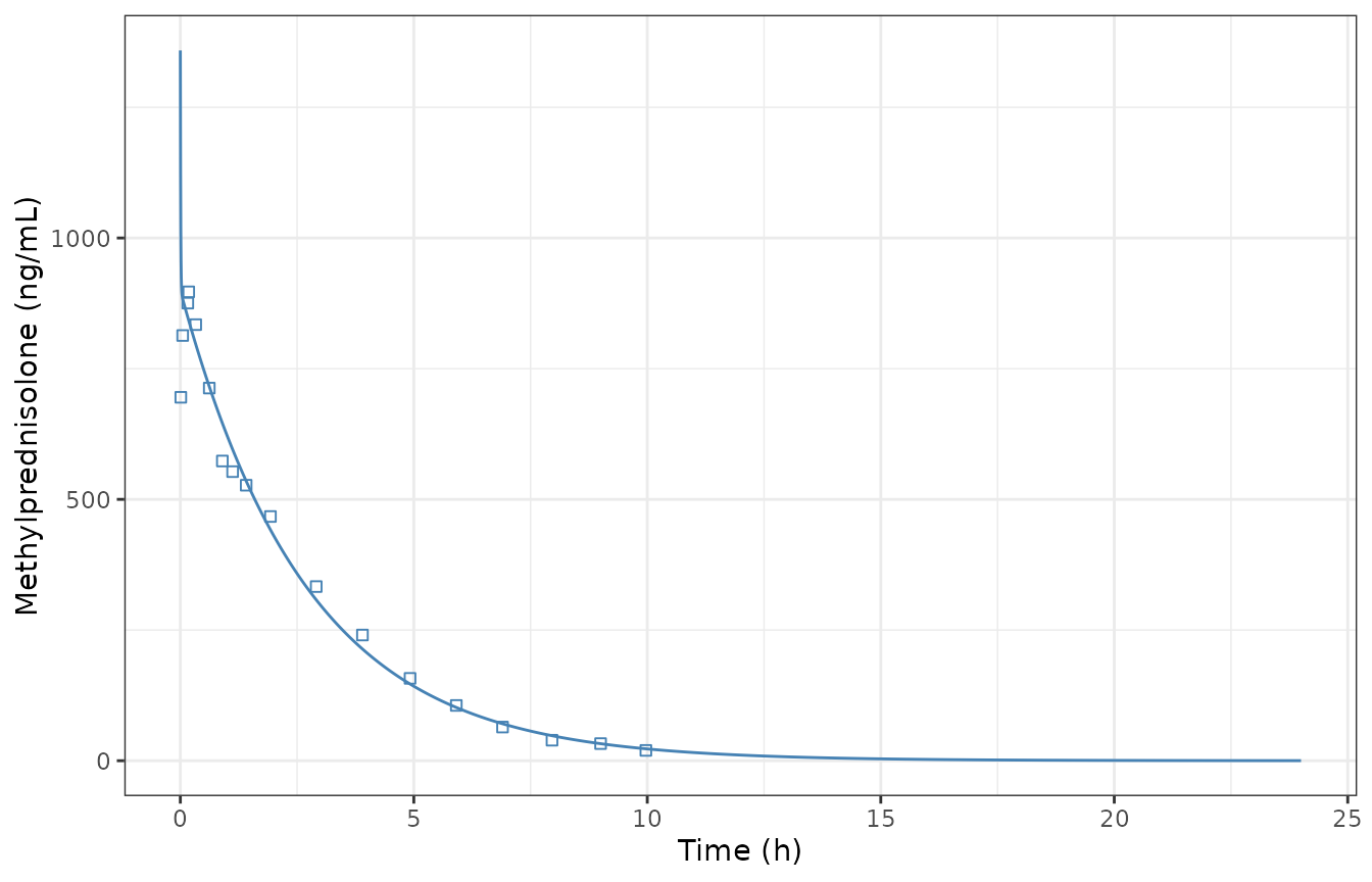
Replicates Supplementary Figure S1 (left) of Cleary 2026: methylprednisolone plasma concentration after an 80 mg intravenous bolus of methylprednisolone sodium succinate in a 70 kg adult (line), with the observed mean profile of in vivo dataset A (squares).
The initial spike reflects distribution that is almost complete within minutes (K12 and K21 of 45 and 89 1/h); after it the profile declines with a half-life of about 1.9 h, as in the paper’s figure.
Checks against the paper
NCA (PKNCA) against Supplementary Table S1
Supplementary Table S1 reports the NCA of the simulated profile: Cmax 842 ng/mL at 0.18 h (used above to derive K21, so not an independent check), AUC0-inf 2443 ngh/mL and AUC0-t 2443 ngh/mL. The paper compares the simulated values with the observed profile at its first sampled peak (0.18 h), since an IV bolus peaks at time zero; the same is done here by computing the simulated Cmax over the observed sampling window.
conc <- sim |> filter(!is.na(Cc_ng))
conc_obj <- PKNCA::PKNCAconc(conc, Cc_ng ~ time | treatment + id)
dose_obj <- PKNCA::PKNCAdose(
  data.frame(treatment = "80 mg IV bolus", id = 1L, time = 0, dose = 80),
  dose ~ time | treatment + id,
  route = "intravascular"
)
intervals <- data.frame(
  start = c(0, 0.18),
  end = c(Inf, 9.97),
  aucinf.obs = c(TRUE, FALSE),
  half.life = c(TRUE, FALSE),
  cmax = c(FALSE, TRUE)
)
nca_res <- PKNCA::pk.nca(PKNCA::PKNCAdata(conc_obj, dose_obj, intervals = intervals))
sim_nca <- as.data.frame(nca_res) |>
  filter(PPTESTCD %in% c("aucinf.obs", "cmax")) |>
  select(treatment, PPTESTCD, PPORRES)

ref_nca <- data.frame(treatment = "80 mg IV bolus", cmax = 842, aucinf.obs = 2443)

cmp <- nlmixr2lib::ncaComparisonTable(
  sim_nca, ref_nca,
  by = "treatment",
  units = c(cmax = "ng/mL", aucinf.obs = "ng*h/mL"),
  tolerance_pct = 20
)
knitr::kable(cmp, caption = attr(cmp, "footnote"))| NCA parameter | treatment | Reference | Simulated | % diff |
|---|---|---|---|---|
| Cmax (ng/mL) | 80 mg IV bolus | 842 | 842 | -0.0% |
| AUC0-∞ (obs) (ng*h/mL) | 80 mg IV bolus | 2440 | 2440 | +0.1% |
The AUC check depends only on clearance (Dose / CL = 80 mg / 32.73 L/h = 2445 ng*h/mL), and so confirms that the paper’s simulation used a 70 kg patient and an 80 mg dose with no salt correction.
auc_sim <- sim_nca$PPORRES[sim_nca$PPTESTCD == "aucinf.obs"]
cmax_sim <- sim_nca$PPORRES[sim_nca$PPTESTCD == "cmax"]
stopifnot(
  # Clearance: AUC0-inf of a linear model is Dose / CL; Table S1 prints
  # 2443 ng*h/mL for the paper's own simulation.
  abs(auc_sim - 2443) / 2443 < 0.01,
  # The K21 back-solve: C(0.18 h) reproduces the printed 842 ng/mL.
  abs(cmax_sim - 842) / 842 < 0.01
)
Fold errors against the observed profile
Supplementary Table S1 also reports the average fold error (AFE, 1.02) and absolute average fold error (AAFE, 1.07) of the simulated profile against dataset A (Equations 1 and 2). Neither was used to derive K21, so they test it, and they also test the reading of Table 1’s ‘Volume of distribution (Vd)’ as the central volume.
events_obs <- bind_rows(
  data.frame(id = 1L, time = 0, amt = 80, evid = 1, cmt = "central", WT = 70),
  data.frame(id = 1L, time = dataset_a$time, amt = 0, evid = 0, cmt = "central", WT = 70)
)
pred <- rxode2::rxSolve(mod, events = events_obs, returnType = "data.frame") |>
  transmute(time, pred = 1000 * Cc) |>
  bind_cols(obs = dataset_a$obs)
afe <- 10^mean(log10(pred$pred / pred$obs))
aafe <- 10^mean(abs(log10(pred$pred / pred$obs)))
data.frame(
  Statistic = c("AFE", "AAFE"),
  "This model" = round(c(afe, aafe), 3),
  "Table S1" = c(1.02, 1.07),
  check.names = FALSE
) |>
knitr::kable(caption = "Fold errors of the simulated profile against in vivo dataset A.")| Statistic | This model | Table S1 |
|---|---|---|
| AFE | 1.034 | 1.02 |
| AAFE | 1.094 | 1.07 |
stopifnot(
  # Both within 0.05 of the printed values; reading Vd as the
  # steady-state volume instead gives an AAFE of 1.64.
  abs(afe - 1.02) < 0.05,
  abs(aafe - 1.07) < 0.05
)
The model reproduces the printed AFE and AAFE to within 0.03. If ‘Volume of distribution (Vd)’ were instead the steady-state volume, the K21 that reproduces 842 ng/mL at 0.18 h would be 2.43 1/h and the AAFE would be 1.64, far from the printed 1.07, so the central-volume reading is the one the paper used.
Assumptions and deviations
- K21 is back-solved. Table 1 prints Vd, CL and K12 for the 2-compartment model but not K21. The value 89.14 1/h is the unique solution that gives the simulated 842 ng/mL at 0.18 h of Supplementary Table S1, and it reproduces the printed AFE and AAFE (see above).
- ‘Volume of distribution (Vd)’ is the central volume. GastroPlus compartmental models are specified by Vc, K12 and K21, and the fold errors rule out the steady-state reading.
- Dose basis. The paper describes the IV dose as 80 mg of methylprednisolone sodium succinate and does not say whether it is expressed as methylprednisolone. The model gives the paper’s simulated AUC with the dose entered as 80 mg, so clearance is relative to the dose as entered.
-
Body-weight scaling. Volume and clearance are per
kg and scale linearly with
WT, with 70 kg as the reference (Table 1). The paper simulated only 70 kg. - The IM layer is not included (see “What this model contains”). The target dissolution profiles of Figure 4, the IM simulations of Figure 3 and the multiple-dose external validation in patients with rheumatoid arthritis (Figure 5) all depend on GastroPlus’s injection-site model, which the paper does not specify.
- No variability. The model was fitted to a mean profile; there are no between-subject or residual variances.
- No erratum was found (CrossRef and Europe PMC, checked 2026-11-12).