Benralizumab (Wang 2017)
Source:vignettes/articles/Wang_2017_benralizumab.Rmd
Wang_2017_benralizumab.Rmd
library(nlmixr2lib)
library(rxode2)
#> rxode2 5.1.2 using 2 threads (see ?getRxThreads)
#>   no cache: create with `rxCreateCache()`
library(dplyr)
#>
#> Attaching package: 'dplyr'
#> The following objects are masked from 'package:stats':
#>
#>     filter, lag
#> The following objects are masked from 'package:base':
#>
#>     intersect, setdiff, setequal, union
library(tidyr)
library(ggplot2)
library(PKNCA)
#>
#> Attaching package: 'PKNCA'
#> The following object is masked from 'package:stats':
#>
#>     filter
Model and source
- Citation: Wang B, Lau YY, Liang M, et al. Population Pharmacokinetics and Pharmacodynamics of Benralizumab in Healthy Volunteers and Patients With Asthma. CPT Pharmacometrics Syst Pharmacol. 2017;6(4):249-257. doi:10.1002/psp4.12160
- Description: Two compartment PK model of benralizumab (anti-IL-5Ralpha) in healthy volunteers and patients with asthma (Wang 2017)
- Article: https://doi.org/10.1002/psp4.12160
Benralizumab population PK simulation
Simulate benralizumab concentration-time profiles using the final population PK model from Wang et al. (2017) in healthy volunteers and patients with asthma (N = 200 across 6 Phase I/II studies).
Benralizumab is a humanized, afucosylated IgG1 monoclonal antibody targeting IL-5 receptor alpha. The model is a 2-compartment model with first-order SC absorption, allometric weight scaling (CL exponent fixed at 0.75), and covariate effects for high-titer anti-drug antibodies (ADA, titer >= 400) on CL and Japanese healthy volunteer status on Vc.
Source: Table 3 of Wang et al. (2017) CPT Pharmacometrics Syst Pharmacol. 6(4):249-257. doi:10.1002/psp4.12160. Parameters verified against PMC5397562.
Dosing dataset
Approved asthma regimen: 30 mg SC every 4 weeks for first 3 doses, then every 8 weeks. Simulate through 30 weeks.
dose_times <- c(0, 28, 56, 112, 168)  # days (weeks 0, 4, 8, 16, 24)

obs_times <- sort(unique(c(
  seq(0, 7, by = 0.5),
  seq(7, 210, by = 3.5)
)))

d_dose <- pop %>%
  crossing(TIME = dose_times) %>%
  mutate(AMT = 30, EVID = 1, CMT = 1, DV = NA_real_)

d_obs <- pop %>%
  crossing(TIME = obs_times) %>%
  mutate(AMT = NA_real_, EVID = 0, CMT = 2, DV = NA_real_)

d_sim <- bind_rows(d_dose, d_obs) %>%
  arrange(ID, TIME, desc(EVID)) %>%
  as.data.frame()
Simulate
mod <- readModelDb("Wang_2017_benralizumab")
conc_unit <- rxode2::rxode(mod)$units[["concentration"]]
#> ℹ parameter labels from comments will be replaced by 'label()'
sim <- rxSolve(mod, d_sim, returnType = "data.frame")
#> ℹ parameter labels from comments will be replaced by 'label()'
Concentration-time profiles
sim_summary <- sim %>%
  filter(time > 0) %>%
  group_by(time) %>%
  summarise(
    median = median(Cc, na.rm = TRUE),
    lo     = quantile(Cc, 0.05, na.rm = TRUE),
    hi     = quantile(Cc, 0.95, na.rm = TRUE),
    .groups = "drop"
  )

ggplot(sim_summary, aes(x = time / 7)) +
  geom_ribbon(aes(ymin = lo, ymax = hi), alpha = 0.2, fill = "darkorange") +
  geom_line(aes(y = median), color = "darkorange", linewidth = 1) +
  labs(
    x = "Time (weeks)",
    y = paste0("Benralizumab concentration (", conc_unit, ")"),
    title = "Simulated benralizumab PK (30 mg SC, q4w x3 then q8w)",
    subtitle = "Median and 90% prediction interval (N = 500 virtual asthma patients)",
    caption = "Model: Wang et al. (2017) CPT Pharmacometrics Syst Pharmacol"
  ) +
  theme_bw()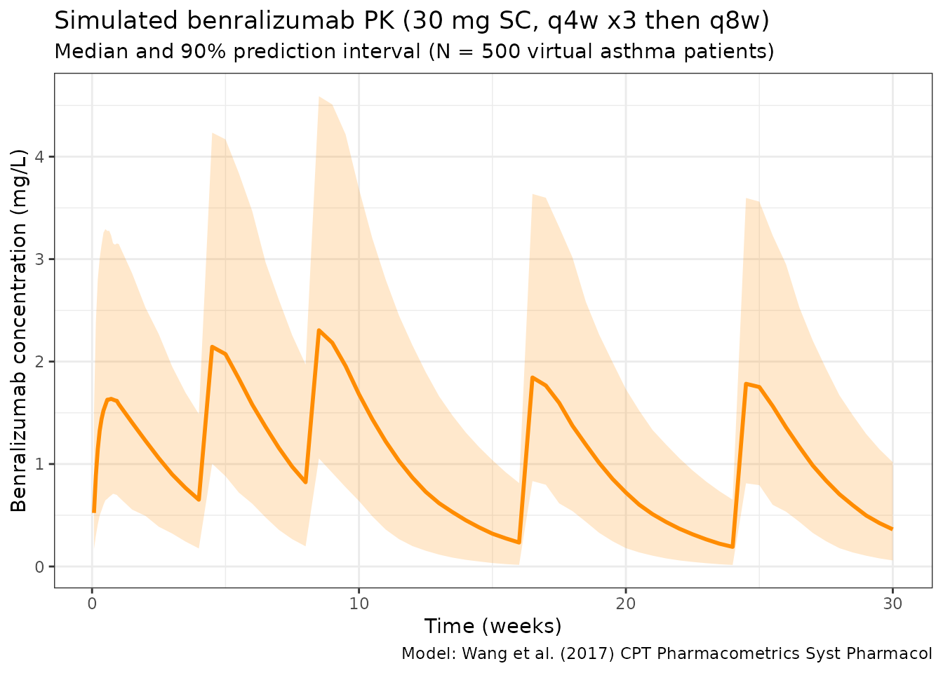
NCA analysis
# Use 2nd dosing interval (weeks 4-8)
sim_df <- as.data.frame(sim)
# Build a unique subject key: use sim.id (replicate) and id (original subject)
# when both are available; otherwise fall back to whichever exists
if (all(c("sim.id", "id") %in% names(sim_df))) {
  sim_df$subject <- paste(sim_df$sim.id, sim_df$id, sep = "_")
} else if ("id" %in% names(sim_df)) {
  sim_df$subject <- sim_df$id
} else {
  sim_df$subject <- sim_df$sim.id
}
sim_df$treatment <- ifelse(sim_df$ADA_POS == 1, "High-titer ADA", "Negative/Low-titer ADA")
nca_data <- data.frame(
  subject   = sim_df$subject,
  treatment = sim_df$treatment,
  time_rel  = sim_df$time - 28,
  Cc        = sim_df$Cc
)
nca_data <- nca_data[nca_data$time_rel >= 0 & nca_data$time_rel <= 28 & nca_data$Cc > 0, ]

conc_obj <- PKNCAconc(nca_data, Cc ~ time_rel | treatment + subject)
dose_obj <- PKNCAdose(
  data.frame(subject = unique(nca_data$subject),
             treatment = nca_data$treatment[match(unique(nca_data$subject), nca_data$subject)],
             time_rel = 0, AMT = 30),
  AMT ~ time_rel | treatment + subject
)
data_obj <- PKNCAdata(conc_obj, dose_obj,
                       intervals = data.frame(start = 0, end = 28,
                                              cmax = TRUE, tmax = TRUE,
                                              auclast = TRUE, half.life = TRUE))
nca_results <- pk.nca(data_obj)
nca_summary <- summary(nca_results)
knitr::kable(nca_summary, digits = 2,
caption = "NCA summary (2nd dosing interval, weeks 4-8)")| start | end | treatment | N | auclast | cmax | tmax | half.life |
|---|---|---|---|---|---|---|---|
| 0 | 28 | High-titer ADA | 21 | 9.63 [49.1] | 0.982 [56.5] | 3.50 [3.50, 3.50] | 5.53 [1.80] |
| 0 | 28 | Negative/Low-titer ADA | 479 | 43.3 [44.9] | 2.29 [42.3] | 3.50 [3.50, 10.5] | 16.1 [5.36] |
Notes
- Model: 2-compartment SC with linear elimination. No TMDD.
- Bioavailability: 52.6% for SC (estimated, not fixed).
- Allometry: CL exponent fixed at 0.75 (standard); Vc and Vp exponents estimated at 0.651 and 0.576 respectively.
- ADA effect: High-titer ADA (>= 400) causes exp(1.52) = 4.57-fold increase in CL (Eq. 6 in paper; Table 3 footnote c “natural exponent”). ADA is time-varying (assessed at each sampling visit).
- Japanese race: 1.34-fold larger Vc for Japanese healthy volunteers (multiplicative factor; may confound with healthy volunteer status).
- IIV on all 6 PK parameters (CL, Vc, Q, Vp, ka, F).
- Reference weight: 77 kg (population mean; paper states “normalized to population median” but exact median not explicitly stated).