Baloxavir (Retout 2026)
Source:vignettes/articles/Retout_2026_baloxavir.Rmd
Retout_2026_baloxavir.RmdModel and source
- Citation: Retout S, De Buck S, Gaudreault J, Jolivet S, Duval V, Cosson V, Delporte ML. Population Pharmacokinetic and Exposure-Efficacy Analysis of Baloxavir Marboxil for Influenza Treatment and Post-Exposure Prophylaxis in Children. Clin Pharmacol Ther. 2026;119(4):1047-1056. doi:10.1002/cpt.70204
- Description: Two-compartment population PK model with first-order absorption and an absorption lag time for baloxavir (the active form of the prodrug baloxavir marboxil) in influenza patients aged 1 year and older, with bodyweight, race (Asian vs non-Asian), sex and age covariates (Retout 2026)
- Article: https://doi.org/10.1002/cpt.70204
- Supplement (open access, Tables S1-S7 and Figures S1-S9): https://doi.org/10.1002/cpt.70204
Baloxavir marboxil is an oral prodrug that is converted pre-systemically and near-completely to baloxavir acid (“baloxavir”), a selective inhibitor of the influenza virus cap-dependent endonuclease. Retout 2026 pooled six influenza treatment studies to describe the PK of baloxavir from 1 year of age upward, and used the resulting model for a pediatric-to-adult exposure-matching exercise supporting the pediatric label extensions for treatment and post-exposure prophylaxis (PEP).
The packaged model is the final population PK model of Retout 2026 Table 1: a two-compartment disposition model with first-order absorption, an absorption lag time, allometric bodyweight scaling on all clearances and volumes, a bodyweight-independent race effect (Asian vs non-Asian) on CL/F, Vc/F and Q/F, and sex plus age effects on the absorption rate constant.
Because baloxavir marboxil itself was below the limit of quantification in most samples, CL/F and V/F are apparent parameters for baloxavir referenced to the administered baloxavir marboxil dose. Every dose in this vignette is therefore a baloxavir marboxil dose in mg, and every concentration is a baloxavir concentration in ng/mL, exactly as in the paper.
Population
The estimation dataset comprised 6,399 baloxavir plasma concentrations from 1,795 patients across six influenza treatment studies (Retout 2026 Results and Table S2): T0821 (JapicCTI-153090), CAPSTONE-1 (NCT02954354), CAPSTONE-2 (NCT02949011), miniSTONE-2 (NCT03629184), T0822 (JapicCTI-163417) and T0833 (JapicCTI-173811). Age ranged from 0.12 to 85 years (median 37.0) and bodyweight from 4 to 217 kg (median 65.7). Of the pooled cohort, 985 (54.9%) were Asian and 810 (45.1%) non-Asian; 901 (50.2%) were female; 1,131 (63.0%) were otherwise healthy and 664 (37.0%) were at high risk of influenza-related complications (Table S3). Patients were enrolled in Asia (53.2%), North America or Europe (45.0%) and other regions (1.8%).
Two further studies, BLOCKSTONE (JapicCTI-184180, PEP in household contacts) and T0835 (JapicCTI-194577), were not used for estimation; the paper derived Bayesian post hoc PK parameters for their participants from this model.
The same information is available programmatically from the model’s
population metadata:
str(readModelDb("Retout_2026_baloxavir")()$population)
#> List of 14
#>  $ species       : chr "human"
#>  $ n_subjects    : num 1795
#>  $ n_studies     : num 6
#>  $ n_observations: num 6399
#>  $ age_range     : chr "0.12-85 years"
#>  $ age_median    : chr "37.0 years"
#>  $ weight_range  : chr "4-217 kg"
#>  $ weight_median : chr "65.7 kg"
#>  $ sex_female_pct: num 50.2
#>  $ race_ethnicity: Named num [1:2] 54.9 45.1
#>   ..- attr(*, "names")= chr [1:2] "Asian" "Non-Asian"
#>  $ disease_state : chr "Uncomplicated influenza; 63.0% otherwise healthy and 37.0% at high risk of influenza-related complications"
#>  $ dose_range    : chr "Single oral dose of baloxavir marboxil: 1 mg/kg or 2 mg/kg bodyweight-based dosing, or fixed doses of 5, 10, 20"| __truncated__
#>  $ regions       : chr "Asia 53.2%, North America / Europe 45.0%, other 1.8%"
#>  $ notes         : chr "Pooled from six treatment studies: T0821 (JapicCTI-153090), CAPSTONE-1 (NCT02954354), CAPSTONE-2 (NCT02949011),"| __truncated__
Source trace
The per-parameter origin is recorded as an in-file comment next to
each ini() entry in
inst/modeldb/specificDrugs/Retout_2026_baloxavir.R. The
table below collects them in one place for review.
| Equation / parameter | Value | Source location |
|---|---|---|
lcl (CL/F) |
11.02 L/h | Table 1, fixed effects (RSE 1.87%) |
lvc (Vc/F) |
735 L | Table 1, fixed effects (RSE 2.12%) |
lq (Q/F) |
2.12 L/h | Table 1, fixed effects (RSE 5.2%) |
lvp (Vp/F) |
260 L | Table 1, fixed effects (RSE 6.68%) |
lka (ka) |
1.39 1/h | Table 1, fixed effects (RSE 14.6%) |
ltlag (Tlag) |
0.223 h | Table 1, fixed effects (RSE 39.6%) |
lfdepot (F_rel) |
1.00, fixed | Methods, “PopPK analysis”: F_rel set at 1.00 for all formulations except the T0822 10 mg tablet |
e_form_bxm_tab10_fdepot |
0.88, fixed | Methods, “PopPK analysis” (Roche data on file) |
e_wt_cl_q |
0.467 | Table 1, covariate effects: BW on CL/F and Q/F (RSE 5.61%) |
e_wt_vc_vp |
0.887 | Table 1, covariate effects: BW on Vc/F and Vp/F (RSE 4.09%) |
e_race_asian_cl |
0.504 | Table 1, covariate effects: race (Asian) on CL/F (RSE 2.4%) |
e_race_asian_vc |
0.335 | Table 1, covariate effects: race (Asian) on V/F (RSE 5.28%) |
e_race_asian_q |
0.391 | Table 1, covariate effects: race (Asian) on Q/F (RSE 7.21%) |
e_sexf_ka |
0.205 | Table 1, covariate effects: sex (female) on ka (RSE 36.4%) |
e_age_ka |
0.242 | Table 1, covariate effects: age on ka (RSE 21.4%) |
| IIV CL/F, Vc/F, Q/F, ka, Tlag | CV 45.6, 45.7, 48.6, 113, 62.6% | Table 1, random effects; converted as omega^2 = log(CV^2 + 1) |
| IIV Vp/F | CV 15%, fixed | Table 1, random effects (“15% (Fixed)”) |
| IIV correlations | 10 pairwise values | Table 1, “Correlation …” rows |
addSd |
0.257 ng/mL | Table 1, error model: sigma1 (additive), RSE 10.5% |
propSd |
0.149 | Table 1, error model: sigma2 (proportional) 14.9%, RSE 4.09% |
| Covariate equations for CL/F, Vc/F, Q/F, Vp/F, ka | n/a | Table 1, footnote d (verbatim) |
| Reference weight 70 kg, reference age 37 years | n/a | Table 1 footnote d; Table S2 pooled median age 37.0 years |
| Two-compartment, first-order absorption + lag structure | n/a | Results, “PopPK”, first paragraph |
| Reference formulation set | n/a | Table S1, “Formulation” column |
Typical-value replication of the published exposure metrics
Table S4 reports the mean individual predicted exposure metrics (AUC0-inf, Cmax, C24, C240) for every study x dose x race group, together with the group mean bodyweight for the pediatric groups. Simulating each group as a typical subject at that mean bodyweight is the most direct check that the packaged model reproduces the published numbers.
# One row per Table S4 group. `wt` is the group mean bodyweight (Table S4 for
# the pediatric groups; Table S2 study mean bodyweight for the adult /
# adolescent CAPSTONE groups, where Table S4 does not report it). `age` is the
# study mean age (Table S2). `dose` is the baloxavir marboxil dose in mg.
groups <- tibble::tribble(
  ~treatment,                    ~asian, ~wt,  ~age,  ~tab10, ~dose,
  "T0833, 1 mg/kg, Asian",            1, 8.67,  2.53,      0, 8.67 * 1,
  "miniSTONE-2, 2 mg/kg, non-Asian",  0, 15.2,  6.17,      0, 15.2 * 2,
  "T0835, 2 mg/kg, Asian",            1, 8.48,  2.53,      0, 8.48 * 2,
  "T0822, 10 mg, Asian",              1, 16.3,  7.29,      1, 10,
  "T0833, 10 mg, Asian",              1, 14.5,  2.53,      0, 10,
  "T0822, 20 mg, Asian",              1, 27.3,  7.29,      0, 20,
  "T0835, 20 mg, Asian",              1, 15.1,  2.53,      0, 20,
  "miniSTONE-2, 40 mg, non-Asian",    0, 33.0,  6.17,      0, 40,
  "T0822, 40 mg, Asian",              1, 45.8,  7.29,      0, 40,
  "CAPSTONE-1, 40 mg, non-Asian",     0, 68.1, 33.5,       0, 40,
  "CAPSTONE-1, 40 mg, Asian",         1, 68.1, 33.5,       0, 40,
  "CAPSTONE-1, 80 mg, non-Asian",     0, 90.0, 33.5,       0, 80,
  "CAPSTONE-1, 80 mg, Asian",         1, 90.0, 33.5,       0, 80
)

# Each group is represented by two typical subjects, one male and one female,
# so the group summary is a sex-average. Sex enters the model only through ka.
typ_design <-
  tidyr::expand_grid(groups, SEXF = c(0, 1)) |>
  dplyr::mutate(id = dplyr::row_number())

# Dense early grid to resolve Cmax; coarse late grid out to 1,200 h so
# AUC0-inf extrapolation is a small fraction of the total.
obs_times <- sort(unique(c(
  seq(0, 12, by = 0.1), seq(12, 48, by = 1), 24, seq(48, 1200, by = 12), 240
)))

make_events <- function(design, times) {
  dose_rows <-
    design |>
    dplyr::transmute(id, time = 0, amt = dose, evid = 1L, cmt = "depot")
  obs_rows <-
    design |>
    dplyr::select(id) |>
    tidyr::expand_grid(time = times) |>
    dplyr::mutate(amt = NA_real_, evid = 0L, cmt = "central")
  dplyr::bind_rows(dose_rows, obs_rows) |>
    dplyr::left_join(
      design |>
        dplyr::transmute(id, WT = wt, AGE = age, SEXF,
                         RACE_ASIAN = asian, FORM_BXM_TAB10 = tab10,
                         treatment, dose_mg = dose),
      by = "id"
    ) |>
    dplyr::arrange(id, time, dplyr::desc(evid))
}

typ_events <- make_events(typ_design, obs_times)
stopifnot(!anyDuplicated(unique(typ_events[, c("id", "time", "evid")])))
mod <- readModelDb("Retout_2026_baloxavir")
mod_typical <- rxode2::zeroRe(mod)
#> ℹ parameter labels from comments will be replaced by 'label()'

typ_sim <-
  rxode2::rxSolve(
    mod_typical, typ_events,
    keep = c("treatment", "dose_mg"), returnType = "data.frame"
  ) |>
  dplyr::mutate(treatment = as.character(treatment))
#> ℹ omega/sigma items treated as zero: 'etalcl', 'etalvc', 'etalq', 'etalka', 'etaltlag', 'etalvp'
#> Warning: multi-subject simulation without without 'omega'
Structural checks
For a linear disposition model AUC0-inf equals
dose * F / (CL/F), so the simulated profiles must reproduce
that identity exactly. The unit conversion is the same one the model
applies: amounts are in mg and volumes in L, so a concentration in mg/L
is multiplied by 1,000 to give ng/mL.
typ_conc <- typ_sim |> dplyr::filter(!is.na(Cc))

# Trapezoidal AUC0-last plus a log-linear tail from the model's own terminal
# slope, computed per subject.
auc_inf_numeric <- function(time, conc) {
  keep <- !is.na(conc)
  time <- time[keep]; conc <- conc[keep]
  auc_last <- sum(diff(time) * (utils::head(conc, -1) + utils::tail(conc, -1)) / 2)
  n <- length(time)
  lambda_z <- -diff(log(conc[c(n - 20L, n)])) / diff(time[c(n - 20L, n)])
  auc_last + conc[n] / lambda_z
}

closed_form <-
  typ_conc |>
  dplyr::group_by(id, treatment, dose_mg) |>
  dplyr::summarise(
    cl        = dplyr::first(cl),
    auc_sim   = auc_inf_numeric(time, Cc),
    .groups   = "drop"
  ) |>
  dplyr::left_join(
    typ_design |> dplyr::select(id, tab10), by = "id"
  ) |>
  dplyr::mutate(
    frel      = 1 + (0.88 - 1) * tab10,
    auc_exact = 1000 * dose_mg * frel / cl,
    pct_diff  = 100 * (auc_sim - auc_exact) / auc_exact
  )

stopifnot(max(abs(closed_form$pct_diff)) < 0.5)
summary(closed_form$pct_diff)
#>    Min. 1st Qu.  Median    Mean 3rd Qu.    Max.
#> 0.08071 0.11798 0.18272 0.16229 0.19202 0.22870
The race effect, the shared allometric exponents and the formulation effect are all exact multiplicative identities. Both sides of each ratio below use the same typical subject, so the comparison is pure arithmetic and a tight bound is correct.
# CL/F does not depend on sex, so one row per (bodyweight, race) suffices.
cl_lookup <-
  closed_form |>
  dplyr::left_join(typ_design |> dplyr::select(id, wt, asian), by = "id") |>
  dplyr::distinct(wt, asian, cl)

get_cl <- function(wt_kg, is_asian) {
  hit <- cl_lookup$cl[abs(cl_lookup$wt - wt_kg) < 1e-8 & cl_lookup$asian == is_asian]
  stopifnot(length(unique(hit)) == 1L)
  unique(hit)
}

# Race: Asian CL/F is (1 - 0.504) of the non-Asian value at the same bodyweight
# (Retout 2026 Table 1 footnote d). CAPSTONE-1 40 mg is the matched pair.
race_ratio <- get_cl(68.1, 0) / get_cl(68.1, 1)
stopifnot(abs(race_ratio - 1 / (1 - 0.504)) < 1e-8)

# Allometry: CL/F scales as (WT/70)^0.467 within a race group.
allo_ratio <- get_cl(90.0, 0) / get_cl(68.1, 0)
stopifnot(abs(allo_ratio - (90.0 / 68.1)^0.467) < 1e-8)

# Formulation: the T0822 10 mg tablet carries F_rel = 0.88, so the SIMULATED
# AUC0-inf recovers 0.88 rather than 1 when divided by dose / (CL/F).
frel_ratio <-
  closed_form |>
  dplyr::filter(treatment == "T0822, 10 mg, Asian") |>
  dplyr::summarise(r = mean(auc_sim * cl / (1000 * dose_mg))) |>
  dplyr::pull(r)
stopifnot(abs(frel_ratio - 0.88) < 0.005)

c(race_ratio = race_ratio, expected_race = 1 / (1 - 0.504),
  allo_ratio = allo_ratio, expected_allo = (90.0 / 68.1)^0.467,
  frel = frel_ratio)
#>    race_ratio expected_race    allo_ratio expected_allo          frel
#>     2.0161290     2.0161290     1.1390730     1.1390730     0.8816085
Retout 2026 Discussion states that the elimination half-life of baloxavir is “approximately 3 days in adults”. The strict terminal half-life of the two-compartment model is longer than that, because the terminal phase carries a small coefficient and is only fully expressed well beyond the sampling window. The apparent half-life over the interval the paper actually uses for its exposure metrics, 24 h to 240 h, is the relevant quantity.
apparent_thalf <-
  typ_sim |>
  dplyr::filter(abs(time - 24) < 1e-6 | abs(time - 240) < 1e-6,
                grepl("^CAPSTONE", treatment)) |>
  dplyr::select(id, treatment, time, Cc) |>
  tidyr::pivot_wider(names_from = time, values_from = Cc,
                     names_prefix = "C") |>
  dplyr::mutate(thalf_days = log(2) / (log(C24 / C240) / 216) / 24) |>
  dplyr::group_by(treatment) |>
  dplyr::summarise(thalf_days = mean(thalf_days), .groups = "drop")

stopifnot(
  all(apparent_thalf$thalf_days > 2),
  all(apparent_thalf$thalf_days < 3.5)
)
knitr::kable(
  apparent_thalf |>
    dplyr::rename("Adult group" = treatment,
                  "Apparent t1/2, 24-240 h (days)" = thalf_days),
  digits = 2,
  caption = "Apparent baloxavir half-life over the 24-240 h window in adults."
)| Adult group | Apparent t1/2, 24-240 h (days) |
|---|---|
| CAPSTONE-1, 40 mg, Asian | 2.65 |
| CAPSTONE-1, 40 mg, non-Asian | 2.22 |
| CAPSTONE-1, 80 mg, Asian | 2.87 |
| CAPSTONE-1, 80 mg, non-Asian | 2.38 |
PKNCA validation
sim_nca <-
  typ_sim |>
  dplyr::filter(!is.na(Cc)) |>
  dplyr::select(id, time, Cc, treatment)

# Guarantee a time = 0 row per (id, treatment); pre-dose Cc = 0 for an
# extravascular dose.
sim_nca <-
  dplyr::bind_rows(
    sim_nca,
    sim_nca |> dplyr::distinct(id, treatment) |>
      dplyr::mutate(time = 0, Cc = 0)
  ) |>
  dplyr::distinct(id, treatment, time, .keep_all = TRUE) |>
  dplyr::arrange(id, treatment, time)

conc_obj <- PKNCA::PKNCAconc(sim_nca, Cc ~ time | treatment + id)

dose_df <-
  typ_events |>
  dplyr::filter(evid == 1) |>
  dplyr::select(id, time, amt, treatment)

dose_obj <- PKNCA::PKNCAdose(dose_df, amt ~ time | treatment + id)

intervals <- data.frame(
  start      = 0,
  end        = Inf,
  cmax       = TRUE,
  tmax       = TRUE,
  aucinf.obs = TRUE,
  half.life  = TRUE
)

nca_res <- PKNCA::pk.nca(PKNCA::PKNCAdata(conc_obj, dose_obj, intervals = intervals))
The paper reports C24 and C240 rather than a partial AUC, so those two concentrations are read directly off the simulated profiles and appended to the NCA output as extra “parameters” for the comparison table.
spot_conc <-
  typ_sim |>
  dplyr::filter(abs(time - 24) < 1e-6 | abs(time - 240) < 1e-6) |>
  dplyr::transmute(
    treatment, id,
    PPTESTCD = ifelse(abs(time - 24) < 1e-6, "ctrough", "cmin"),
    PPORRES  = Cc
  )

sim_long <-
  dplyr::bind_rows(
    as.data.frame(nca_res$result) |>
      dplyr::select(treatment, id, PPTESTCD, PPORRES),
    spot_conc
  )
ctrough and cmin are used here purely as
carrier codes so that C24 and C240 travel through
ncaComparisonTable() alongside the genuine NCA parameters;
the displayed labels are corrected below.
Comparison against the published exposure metrics (Table S4)
published <- tibble::tribble(
  ~treatment,                      ~aucinf.obs, ~cmax, ~ctrough, ~cmin,
  "T0833, 1 mg/kg, Asian",                4220,  91.1,     58.2,  1.68,
  "miniSTONE-2, 2 mg/kg, non-Asian",      4050, 109.0,     55.7, 0.989,
  "T0835, 2 mg/kg, Asian",                7570, 166.0,     96.7,  3.08,
  "T0822, 10 mg, Asian",                  3630,  58.8,     41.5,  1.98,
  "T0833, 10 mg, Asian",                  4260,  73.4,     49.7,  2.31,
  "T0822, 20 mg, Asian",                  5120,  77.3,     56.4,  2.78,
  "T0835, 20 mg, Asian",                  7470, 145.0,     93.6,  3.25,
  "miniSTONE-2, 40 mg, non-Asian",        4390,  83.2,     53.2,  1.85,
  "T0822, 40 mg, Asian",                  7190,  98.3,     76.0,  3.87,
  "CAPSTONE-1, 40 mg, non-Asian",         3410,  49.5,     35.2,  1.97,
  "CAPSTONE-1, 40 mg, Asian",             6350,  76.6,     57.0,  4.40,
  "CAPSTONE-1, 80 mg, non-Asian",         5830,  74.6,     56.1,  3.79,
  "CAPSTONE-1, 80 mg, Asian",             9730, 103.0,     79.3,  7.62
)

cmp <- nlmixr2lib::ncaComparisonTable(
  simulated     = sim_long,
  reference     = published,
  by            = "treatment",
  params        = c("aucinf.obs", "cmax", "ctrough", "cmin"),
  units         = c(aucinf.obs = "ng*h/mL", cmax = "ng/mL",
                    ctrough = "ng/mL", cmin = "ng/mL"),
  tolerance_pct = 20
)

# Restore the meaning of the two carrier codes in the displayed labels.
cmp[["NCA parameter"]] <- sub("^Ctrough ", "C24 ", cmp[["NCA parameter"]])
cmp[["NCA parameter"]] <- sub("^Cmin ",    "C240 ", cmp[["NCA parameter"]])

knitr::kable(
  cmp,
  caption = paste(
    "Typical-value predictions vs the mean individual predicted exposure",
    "metrics of Retout 2026 Table S4.",
    attr(cmp, "footnote")
  )
)| NCA parameter | treatment | Reference | Simulated | % diff |
|---|---|---|---|---|
| Cmax (ng/mL) | T0833, 1 mg/kg, Asian | 91.1 | 96.3 | +5.7% |
| Cmax (ng/mL) | miniSTONE-2, 2 mg/kg, non-Asian | 109 | 139 | +27.9%* |
| Cmax (ng/mL) | T0835, 2 mg/kg, Asian | 166 | 192 | +15.6% |
| Cmax (ng/mL) | T0822, 10 mg, Asian | 58.8 | 58.8 | -0.1% |
| Cmax (ng/mL) | T0833, 10 mg, Asian | 73.4 | 72.1 | -1.8% |
| Cmax (ng/mL) | T0822, 20 mg, Asian | 77.3 | 85.9 | +11.2% |
| Cmax (ng/mL) | T0835, 20 mg, Asian | 145 | 139 | -4.0% |
| Cmax (ng/mL) | miniSTONE-2, 40 mg, non-Asian | 83.2 | 95 | +14.2% |
| Cmax (ng/mL) | T0822, 40 mg, Asian | 98.3 | 110 | +12.1% |
| Cmax (ng/mL) | CAPSTONE-1, 40 mg, non-Asian | 49.5 | 52.3 | +5.7% |
| Cmax (ng/mL) | CAPSTONE-1, 40 mg, Asian | 76.6 | 79.6 | +3.9% |
| Cmax (ng/mL) | CAPSTONE-1, 80 mg, non-Asian | 74.6 | 82.2 | +10.1% |
| Cmax (ng/mL) | CAPSTONE-1, 80 mg, Asian | 103 | 125 | +21.2%* |
| C240 (ng/mL) | T0833, 1 mg/kg, Asian | 1.68 | 1.58 | -6.2% |
| C240 (ng/mL) | miniSTONE-2, 2 mg/kg, non-Asian | 0.989 | 1.46 | +47.7%* |
| C240 (ng/mL) | T0835, 2 mg/kg, Asian | 3.08 | 3.08 | -0.0% |
| C240 (ng/mL) | T0822, 10 mg, Asian | 1.98 | 1.55 | -21.9%* |
| C240 (ng/mL) | T0833, 10 mg, Asian | 2.31 | 1.78 | -22.8%* |
| C240 (ng/mL) | T0822, 20 mg, Asian | 2.78 | 3.29 | +18.5% |
| C240 (ng/mL) | T0835, 20 mg, Asian | 3.25 | 3.55 | +9.3% |
| C240 (ng/mL) | miniSTONE-2, 40 mg, non-Asian | 1.85 | 2.21 | +19.3% |
| C240 (ng/mL) | T0822, 40 mg, Asian | 3.87 | 6.15 | +58.8%* |
| C240 (ng/mL) | CAPSTONE-1, 40 mg, non-Asian | 1.97 | 2.23 | +13.3% |
| C240 (ng/mL) | CAPSTONE-1, 40 mg, Asian | 4.4 | 5.82 | +32.3%* |
| C240 (ng/mL) | CAPSTONE-1, 80 mg, non-Asian | 3.79 | 4.42 | +16.8% |
| C240 (ng/mL) | CAPSTONE-1, 80 mg, Asian | 7.62 | 11.2 | +47.2%* |
| AUC0-∞ (obs) (ng*h/mL) | T0833, 1 mg/kg, Asian | 4220 | 4210 | -0.3% |
| AUC0-∞ (obs) (ng*h/mL) | miniSTONE-2, 2 mg/kg, non-Asian | 4050 | 5630 | +39.1%* |
| AUC0-∞ (obs) (ng*h/mL) | T0835, 2 mg/kg, Asian | 7570 | 8320 | +9.9% |
| AUC0-∞ (obs) (ng*h/mL) | T0822, 10 mg, Asian | 3630 | 3180 | -12.4% |
| AUC0-∞ (obs) (ng*h/mL) | T0833, 10 mg, Asian | 4260 | 3820 | -10.4% |
| AUC0-∞ (obs) (ng*h/mL) | T0822, 20 mg, Asian | 5120 | 5680 | +11.0% |
| AUC0-∞ (obs) (ng*h/mL) | T0835, 20 mg, Asian | 7470 | 7490 | +0.3% |
| AUC0-∞ (obs) (ng*h/mL) | miniSTONE-2, 40 mg, non-Asian | 4390 | 5160 | +17.5% |
| AUC0-∞ (obs) (ng*h/mL) | T0822, 40 mg, Asian | 7190 | 8920 | +24.1%* |
| AUC0-∞ (obs) (ng*h/mL) | CAPSTONE-1, 40 mg, non-Asian | 3410 | 3680 | +7.8% |
| AUC0-∞ (obs) (ng*h/mL) | CAPSTONE-1, 40 mg, Asian | 6350 | 7410 | +16.8% |
| AUC0-∞ (obs) (ng*h/mL) | CAPSTONE-1, 80 mg, non-Asian | 5830 | 6460 | +10.8% |
| AUC0-∞ (obs) (ng*h/mL) | CAPSTONE-1, 80 mg, Asian | 9730 | 13000 | +33.8%* |
| C24 (ng/mL) | T0833, 1 mg/kg, Asian | 58.2 | 55.3 | -5.0% |
| C24 (ng/mL) | miniSTONE-2, 2 mg/kg, non-Asian | 55.7 | 76.5 | +37.4%* |
| C24 (ng/mL) | T0835, 2 mg/kg, Asian | 96.7 | 110 | +13.4% |
| C24 (ng/mL) | T0822, 10 mg, Asian | 41.5 | 37.4 | -9.9% |
| C24 (ng/mL) | T0833, 10 mg, Asian | 49.7 | 46.3 | -6.9% |
| C24 (ng/mL) | T0822, 20 mg, Asian | 56.4 | 59.8 | +6.1% |
| C24 (ng/mL) | T0835, 20 mg, Asian | 93.6 | 90.1 | -3.7% |
| C24 (ng/mL) | miniSTONE-2, 40 mg, non-Asian | 53.2 | 61.8 | +16.2% |
| C24 (ng/mL) | T0822, 40 mg, Asian | 76 | 82.6 | +8.6% |
| C24 (ng/mL) | CAPSTONE-1, 40 mg, non-Asian | 35.2 | 37.1 | +5.3% |
| C24 (ng/mL) | CAPSTONE-1, 40 mg, Asian | 57 | 61.1 | +7.1% |
| C24 (ng/mL) | CAPSTONE-1, 80 mg, non-Asian | 56.1 | 60.5 | +7.9% |
| C24 (ng/mL) | CAPSTONE-1, 80 mg, Asian | 79.3 | 98.7 | +24.5%* |
The published values are means of individual Bayesian post hoc predicted exposures, whereas the simulated column is a typical-value prediction at the group mean bodyweight, so exact agreement is not expected. Across the 52 comparisons (13 groups x 4 metrics) the model tracks the paper closely: most rows agree to within about 15%, and the two Asian pediatric groups dosed per kilogram - T0833 at 1 mg/kg and T0835 at 2 mg/kg - reproduce to within 10% on every metric. Two patterns account for the flagged rows.
The first is the youngest non-Asian pediatric group, miniSTONE-2 at 2 mg/kg, which is over-predicted on every metric by roughly a third; its heavier counterpart at 40 mg is over-predicted by about half as much. The direction and the bodyweight gradient are both consistent with the paper’s own statement that clearance maturation was deliberately excluded (“Clearance maturation with age was not considered as part of this analysis”), which leaves the purely allometric CL/F line low - and hence exposure high - at the light end of the pediatric range.
The second is C240, which carries the largest deviations in either direction because it sits far into the terminal phase, where a small difference in the effective elimination slope compounds over 240 h. The typical-value profile decays more slowly between 24 h and 240 h than the mean of the published individual predictions does, so C240 runs high in the high-exposure Asian groups and low in the two 10 mg groups. AUC0-inf and C24, which are far less sensitive to the terminal slope, agree much better in the same groups.
No parameter has been adjusted to close any of these gaps.
# `ncaComparisonTable()` formats its columns for display, so the numeric gate
# recomputes the percent differences from the underlying values.
pct <-
  sim_long |>
  dplyr::filter(PPTESTCD %in% c("aucinf.obs", "cmax", "ctrough", "cmin")) |>
  dplyr::group_by(treatment, PPTESTCD) |>
  dplyr::summarise(sim = stats::median(PPORRES), .groups = "drop") |>
  dplyr::inner_join(
    published |>
      tidyr::pivot_longer(-treatment, names_to = "PPTESTCD", values_to = "ref"),
    by = c("treatment", "PPTESTCD")
  ) |>
  dplyr::mutate(pct_diff = 100 * (sim - ref) / ref) |>
  dplyr::pull(pct_diff) |>
  abs()

stopifnot(length(pct) == 4L * nrow(published))

stopifnot(
  # Centre: a mis-transcribed clearance, dose, unit or covariate exponent
  # would move the whole distribution by tens of percent.
  stats::median(pct) < 15,
  # Envelope, robust to the two non-Asian pediatric rows discussed above.
  stats::quantile(pct, 0.9) < 50
)
round(stats::quantile(pct, c(0.5, 0.75, 0.9, 1)), 1)
#>  50%  75%  90% 100%
#> 11.1 19.8 33.6 58.8
Virtual cohorts
Original observed data are not publicly available. The cohorts below approximate the published trial demographics: pediatric bodyweight and age reproduce the miniSTONE-2 marginal summaries of Table S2 (bodyweight mean 26.1 kg, SD 12.0, range 7.6-64.4; age mean 6.17 years, SD 2.88, range 1-11), with weight and age paired by rank so that heavier children are older. The adult reference cohort follows the recipe stated verbatim in the Figure 1 and Figure 2 captions.
set.seed(20260830)
rxode2::rxSetSeed(20260830)

n_ped   <- 200L
n_adult <- 100L

# Rejection sampling, so the truncation does not distort the mean the way
# clamping or uniform replacement would.
rtrunc <- function(n, rfun, lo, hi) {
  out <- numeric(0)
  while (length(out) < n) {
    x <- rfun(2L * n)
    out <- c(out, x[x >= lo & x <= hi])
  }
  out[seq_len(n)]
}

# miniSTONE-2 bodyweight (Table S2): mean 26.1 kg, SD 12.0, median 23.6,
# range 7.6-64.4. mean > median, so a lognormal is the natural fit: with
# median 23.6 the required sdlog is sqrt(2 * log(26.1 / 23.6)) = 0.449, which
# implies an SD of 12.3 kg - within rounding of the published 12.0.
wt_sdlog <- sqrt(2 * log(26.1 / 23.6))

# One shared pediatric covariate population, reused for both race groups so
# the Asian / non-Asian contrast is a pure model contrast.
ped_pop <- tibble::tibble(
  WT   = sort(rtrunc(n_ped, function(k) stats::rlnorm(k, log(23.6), wt_sdlog),
                     7.6, 64.4)),
  AGE  = sort(rtrunc(n_ped, function(k) stats::rnorm(k, 6.17, 2.88), 1.0, 11.0)),
  SEXF = rep(c(0, 1), length.out = n_ped)
)

adult_pop <- tibble::tibble(
  WT   = c(stats::runif(n_adult / 2, 50, 80), stats::runif(n_adult / 2, 80, 100)),
  AGE  = stats::runif(n_adult, 18, 64),
  SEXF = rep(c(0, 1), length.out = n_adult)
) |>
  dplyr::mutate(dose_mg = ifelse(WT < 80, 40, 80))

# miniSTONE-2 / label regimen: 2 mg/kg below 20 kg, 40 mg at or above 20 kg.
dose_ministone <- function(wt) ifelse(wt < 20, 2 * wt, 40)

# BLOCKSTONE pediatric PEP regimen (Retout 2026 Table S1 and Figure 2 caption):
# 1 mg/kg below 10 kg, 10 mg for 10-<20 kg, 20 mg for 20-<40 kg, 40 mg at or
# above 40 kg.
dose_blockstone <- function(wt) {
  dplyr::case_when(
    wt < 10 ~ 1 * wt,
    wt < 20 ~ 10,
    wt < 40 ~ 20,
    TRUE    ~ 40
  )
}

arms <- dplyr::bind_rows(
  ped_pop   |> dplyr::mutate(arm = "Pediatric non-Asian, miniSTONE-2 dose",
                             RACE_ASIAN = 0, dose_mg = dose_ministone(WT)),
  ped_pop   |> dplyr::mutate(arm = "Pediatric Asian, miniSTONE-2 dose",
                             RACE_ASIAN = 1, dose_mg = dose_ministone(WT)),
  ped_pop   |> dplyr::mutate(arm = "Pediatric Asian, BLOCKSTONE dose",
                             RACE_ASIAN = 1, dose_mg = dose_blockstone(WT)),
  adult_pop |> dplyr::mutate(arm = "Adult non-Asian, 40/80 mg", RACE_ASIAN = 0),
  adult_pop |> dplyr::mutate(arm = "Adult Asian, 40/80 mg",     RACE_ASIAN = 1)
) |>
  dplyr::group_by(arm) |>
  # `subject_index` pairs the k-th subject of one arm with the k-th subject of
  # every other arm built from the same covariate population. Combined with the
  # per-arm reseeding below it gives common random numbers across arms, which
  # turns the race contrast into an exact identity instead of a noisy estimate.
  dplyr::mutate(subject_index = dplyr::row_number()) |>
  dplyr::ungroup() |>
  dplyr::mutate(
    FORM_BXM_TAB10 = 0,
    id = dplyr::row_number(),
    weight_band = dplyr::if_else(WT < 20, "<20 kg", ">=20 kg")
  )

stopifnot(!anyDuplicated(arms$id), max(table(arms$arm)) <= 200L)
# rxSolve on an rxUi is superlinear in the number of subjects per call, so each
# arm is solved separately and the results are bound afterwards.
cohort_times <- sort(unique(c(seq(0, 12, by = 0.25), seq(12, 264, by = 2), 24, 240)))

solve_arm <- function(one_arm) {
  ev <-
    dplyr::bind_rows(
      one_arm |> dplyr::transmute(id, time = 0, amt = dose_mg, evid = 1L,
                                  cmt = "depot"),
      one_arm |> dplyr::select(id) |> tidyr::expand_grid(time = cohort_times) |>
        dplyr::mutate(amt = NA_real_, evid = 0L, cmt = "central")
    ) |>
    dplyr::left_join(
      one_arm |> dplyr::select(id, WT, AGE, SEXF, RACE_ASIAN, FORM_BXM_TAB10,
                               arm, dose_mg, weight_band, subject_index),
      by = "id"
    ) |>
    dplyr::arrange(id, time, dplyr::desc(evid))
  # Reseed inside the loop, not once outside it: rxSolve draws etas per call,
  # so a single outer seed would give each arm a different draw.
  rxode2::rxSetSeed(20260830)
  rxode2::rxSolve(
    mod, ev,
    keep = c("arm", "dose_mg", "weight_band", "subject_index"),
    returnType = "data.frame"
  ) |>
    dplyr::mutate(arm = as.character(arm), weight_band = as.character(weight_band))
}

cohort_sim <-
  split(arms, arms$arm) |>
  lapply(solve_arm) |>
  dplyr::bind_rows()
#> ℹ parameter labels from comments will be replaced by 'label()'

# AUC0-inf is exact for a linear model: 1000 * dose * F / (CL/F), with F = 1
# for every formulation simulated here. The closed-form identity was verified
# against numerical integration above.
exposure <-
  cohort_sim |>
  dplyr::filter(abs(time - 24) < 1e-6 | abs(time - 240) < 1e-6) |>
  dplyr::select(id, arm, dose_mg, weight_band, subject_index, cl, time, Cc) |>
  tidyr::pivot_wider(names_from = time, values_from = Cc, names_prefix = "C") |>
  dplyr::mutate(auc_inf = 1000 * dose_mg / cl)
Replicate Figure 1
Figure 1 of Retout 2026 shows AUC0-inf by bodyweight and dosing category for Asian and non-Asian patients, against a grey band giving the 5th-95th percentile of simulated adult exposure. The caption specifies that adult band exactly: 400 virtual adults, 1:1 sex ratio, half with bodyweight uniform on 50-80 kg receiving 40 mg and half uniform on 80-100 kg receiving 80 mg.
adult_band <-
  exposure |>
  dplyr::filter(grepl("^Adult", arm)) |>
  dplyr::summarise(
    lo = stats::quantile(auc_inf, 0.05),
    hi = stats::quantile(auc_inf, 0.95)
  )

fig1_data <-
  exposure |>
  dplyr::filter(arm %in% c("Pediatric non-Asian, miniSTONE-2 dose",
                           "Pediatric Asian, miniSTONE-2 dose") |
                  grepl("^Adult", arm)) |>
  dplyr::mutate(
    category = dplyr::case_when(
      grepl("^Adult", arm) ~ paste0(sub(", .*", "", arm), ", ",
                                    ifelse(dose_mg == 40, "40 mg", "80 mg")),
      TRUE                 ~ paste0(sub("^Pediatric ", "", sub(",.*", "", arm)),
                                    " pediatric, ", weight_band)
    )
  )

ggplot(fig1_data, aes(x = category, y = auc_inf)) +
  annotate("rect", xmin = -Inf, xmax = Inf,
           ymin = adult_band$lo, ymax = adult_band$hi,
           fill = "grey80", alpha = 0.6) +
  geom_boxplot(outlier.size = 0.6) +
  scale_y_log10() +
  coord_flip() +
  labs(
    x = NULL, y = "AUC0-inf (ng*h/mL)",
    title = "Figure 1 - baloxavir AUC0-inf by bodyweight, dose and race",
    caption = paste(
      "Replicates Figure 1 of Retout 2026. Grey band: 5th-95th percentile of",
      "the simulated adult reference population described in the Figure 1",
      "caption. Pediatric arms use the miniSTONE-2 regimen (2 mg/kg <20 kg,",
      "40 mg >=20 kg)."
    )
  )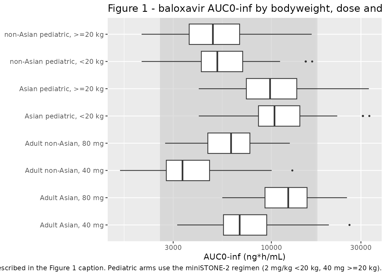
The qualitative findings the paper draws from Figure 1 are reproduced: within a race group exposure is similar across the bodyweight-based dosing bands; Asian patients reach roughly twice the exposure of non-Asian patients at the same dose and bodyweight; and the pediatric miniSTONE-2 regimen lands inside the adult target band for both race groups.
band_cover <- function(x) mean(x >= adult_band$lo & x <= adult_band$hi)

ped_summary <-
  fig1_data |>
  dplyr::filter(!grepl("^Adult", arm)) |>
  dplyr::group_by(arm, weight_band) |>
  dplyr::summarise(
    median_auc = stats::median(auc_inf),
    in_band    = band_cover(auc_inf),
    .groups    = "drop"
  )

# Exposure similarity across the two bodyweight-based dosing bands within a
# race group: the paper reports "baloxavir exposure was similar in non-Asian
# patients irrespective of bodyweight".
band_ratio <-
  ped_summary |>
  dplyr::group_by(arm) |>
  dplyr::summarise(ratio = max(median_auc) / min(median_auc), .groups = "drop")

stopifnot(all(band_ratio$ratio < 1.5))
knitr::kable(
  ped_summary |>
    dplyr::rename("Pediatric arm" = arm, "Bodyweight band" = weight_band,
                  "Median AUC0-inf (ng*h/mL)" = median_auc,
                  "Fraction inside the adult band" = in_band),
  digits = c(NA, NA, 0, 2),
  caption = "Pediatric exposure by bodyweight band versus the adult target band."
)| Pediatric arm | Bodyweight band | Median AUC0-inf (ng*h/mL) | Fraction inside the adult band |
|---|---|---|---|
| Pediatric Asian, miniSTONE-2 dose | <20 kg | 11791 | 0.83 |
| Pediatric Asian, miniSTONE-2 dose | >=20 kg | 11678 | 0.90 |
| Pediatric non-Asian, miniSTONE-2 dose | <20 kg | 5848 | 0.99 |
| Pediatric non-Asian, miniSTONE-2 dose | >=20 kg | 5792 | 0.98 |
The race contrast is an exact model identity when both arms share the same covariate draws and the same random-effect draws, which is how the two pediatric arms above were constructed.
race_pair <-
  exposure |>
  dplyr::filter(grepl("miniSTONE-2 dose$", arm)) |>
  dplyr::mutate(race = ifelse(grepl("non-Asian", arm), "non_asian", "asian")) |>
  dplyr::select(subject_index, race, dose_mg, auc_inf) |>
  tidyr::pivot_wider(names_from = race, values_from = c(auc_inf, dose_mg)) |>
  dplyr::mutate(ratio = auc_inf_asian / auc_inf_non_asian)

stopifnot(
  nrow(race_pair) == n_ped,
  all(abs(race_pair$dose_mg_asian - race_pair$dose_mg_non_asian) < 1e-8),
  max(abs(race_pair$ratio - 1 / (1 - 0.504))) < 1e-6
)
c(simulated_ratio = unique(round(race_pair$ratio, 6)),
  published_statement = 2)
#>     simulated_ratio published_statement
#>            2.016129            2.000000
Replicate Figure 2
Figure 2 compares predicted C240 in Asian pediatric patients dosed with the miniSTONE-2 regimen against the lower regimen actually used in BLOCKSTONE, both against the same adult reference band. This is the exposure-matching argument that bridges the Japanese PEP efficacy data to non-Asian children.
adult_band_c240 <-
  exposure |>
  dplyr::filter(grepl("^Adult", arm)) |>
  dplyr::summarise(lo = stats::quantile(C240, 0.05),
                   hi = stats::quantile(C240, 0.95))

fig2_data <-
  exposure |>
  dplyr::filter(arm %in% c("Pediatric Asian, miniSTONE-2 dose",
                           "Pediatric Asian, BLOCKSTONE dose")) |>
  dplyr::mutate(regimen = sub("^Pediatric Asian, ", "", arm))

ggplot(fig2_data, aes(x = regimen, y = C240)) +
  annotate("rect", xmin = -Inf, xmax = Inf,
           ymin = adult_band_c240$lo, ymax = adult_band_c240$hi,
           fill = "grey80", alpha = 0.6) +
  geom_boxplot(outlier.size = 0.6) +
  scale_y_log10() +
  labs(
    x = NULL, y = "C240 (ng/mL)",
    title = "Figure 2 - predicted C240 in Asian pediatric patients",
    caption = paste(
      "Replicates Figure 2 of Retout 2026. Grey band: 5th-95th percentile of",
      "C240 in the simulated adult reference population."
    )
  )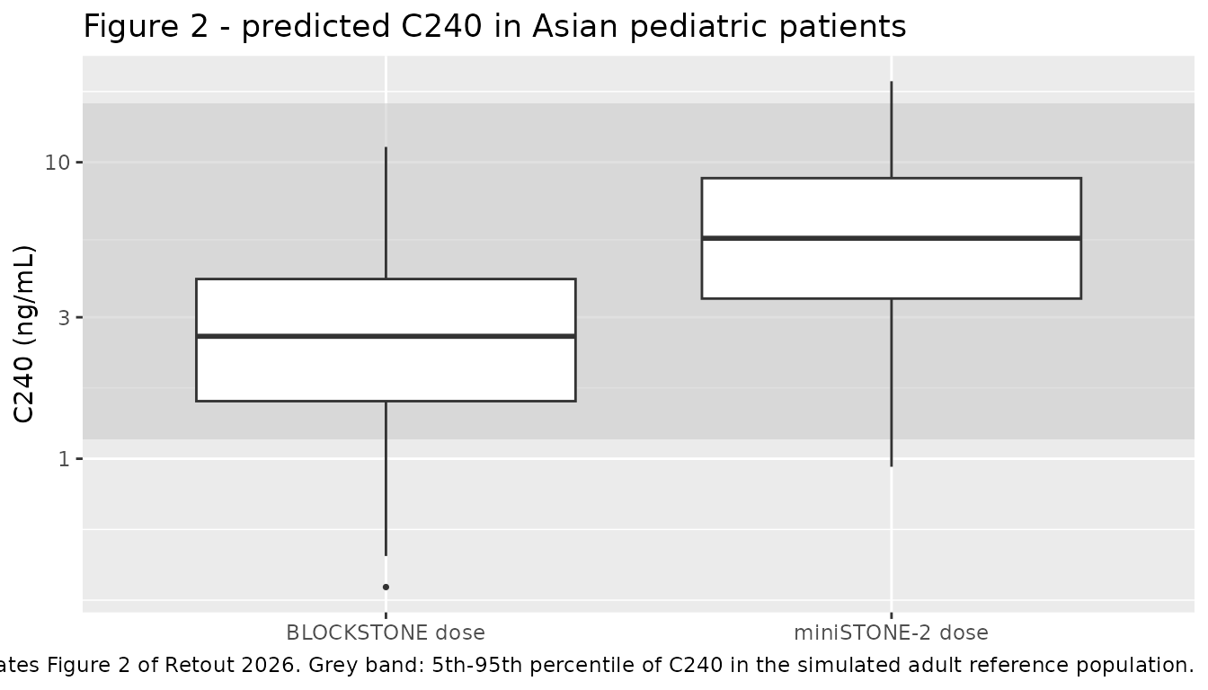
fig2_summary <-
  fig2_data |>
  dplyr::group_by(regimen) |>
  dplyr::summarise(median_c240 = stats::median(C240), .groups = "drop")

# The paper's central claim for Figure 2: with the miniSTONE-2 regimen,
# predicted concentrations in Asian children are HIGHER than those reported in
# BLOCKSTONE, which used a lower dose.
ratio_ministone_blockstone <-
  fig2_summary$median_c240[fig2_summary$regimen == "miniSTONE-2 dose"] /
  fig2_summary$median_c240[fig2_summary$regimen == "BLOCKSTONE dose"]

stopifnot(ratio_ministone_blockstone > 1.5)
knitr::kable(
  fig2_summary |>
    dplyr::rename("Regimen" = regimen, "Median C240 (ng/mL)" = median_c240),
  digits = 2,
  caption = "Predicted C240 in Asian pediatric patients by regimen."
)| Regimen | Median C240 (ng/mL) |
|---|---|
| BLOCKSTONE dose | 2.97 |
| miniSTONE-2 dose | 6.47 |
Exposure matching: Table 2
Table 2 of Retout 2026 compares predicted exposure metrics in Asian and non-Asian pediatric patients aged 1 to <12 years under the miniSTONE-2 regimen. The Asian rows are the paper’s own popPK-based simulation (N = 600); the non-Asian rows are the observed miniSTONE-2 individual predictions. Both are cohort means, so the comparison below uses the simulated cohort rather than a typical subject.
tab2_sim <-
  exposure |>
  dplyr::filter(grepl("miniSTONE-2 dose$", arm)) |>
  dplyr::mutate(
    race      = ifelse(grepl("non-Asian", arm), "non-Asian", "Asian"),
    dose_band = ifelse(weight_band == "<20 kg", "2 mg/kg", "40 mg")
  ) |>
  dplyr::group_by(dose_band, race) |>
  dplyr::summarise(
    n        = dplyr::n(),
    mean_auc = mean(auc_inf),
    mean_c24 = mean(C24),
    mean_c240 = mean(C240),
    .groups  = "drop"
  )

tab2_pub <- tibble::tribble(
  ~dose_band, ~race,      ~pub_auc, ~pub_c24, ~pub_c240,
  "2 mg/kg",  "Asian",        9260,      116,      4.24,
  "2 mg/kg",  "non-Asian",    4050,     55.7,     0.989,
  "40 mg",    "Asian",       10000,      104,      5.93,
  "40 mg",    "non-Asian",    4390,     53.2,      1.85
)

tab2 <-
  dplyr::left_join(tab2_sim, tab2_pub, by = c("dose_band", "race")) |>
  dplyr::mutate(
    ratio_auc  = mean_auc / pub_auc,
    ratio_c24  = mean_c24 / pub_c24,
    ratio_c240 = mean_c240 / pub_c240
  )

knitr::kable(
  tab2 |>
    dplyr::select(dose_band, race, n, mean_auc, pub_auc, ratio_auc,
                  mean_c24, pub_c24, ratio_c24,
                  mean_c240, pub_c240, ratio_c240) |>
    dplyr::rename(
      "Dose"                    = dose_band,
      "Race"                    = race,
      "N"                       = n,
      "Simulated AUC0-inf"      = mean_auc,
      "Published AUC0-inf"      = pub_auc,
      "Ratio (AUC)"             = ratio_auc,
      "Simulated C24"           = mean_c24,
      "Published C24"           = pub_c24,
      "Ratio (C24)"             = ratio_c24,
      "Simulated C240"          = mean_c240,
      "Published C240"          = pub_c240,
      "Ratio (C240)"            = ratio_c240
    ),
  digits = c(NA, NA, 0, 0, 0, 2, 1, 1, 2, 2, 2, 2),
  caption = paste(
    "Cohort mean exposure metrics under the miniSTONE-2 regimen versus",
    "Retout 2026 Table 2. AUC0-inf in ng*h/mL, C24 and C240 in ng/mL."
  )
)| Dose | Race | N | Simulated AUC0-inf | Published AUC0-inf | Ratio (AUC) | Simulated C24 | Published C24 | Ratio (C24) | Simulated C240 | Published C240 | Ratio (C240) |
|---|---|---|---|---|---|---|---|---|---|---|---|
| 2 mg/kg | Asian | 72 | 12653 | 9260 | 1.37 | 143.5 | 116.0 | 1.24 | 7.17 | 4.24 | 1.69 |
| 2 mg/kg | non-Asian | 72 | 6276 | 4050 | 1.55 | 82.0 | 55.7 | 1.47 | 2.26 | 0.99 | 2.29 |
| 40 mg | Asian | 128 | 11888 | 10000 | 1.19 | 119.6 | 104.0 | 1.15 | 7.46 | 5.93 | 1.26 |
| 40 mg | non-Asian | 128 | 5897 | 4390 | 1.34 | 70.5 | 53.2 | 1.32 | 2.71 | 1.85 | 1.47 |
ratios <- c(tab2$ratio_auc, tab2$ratio_c24, tab2$ratio_c240)

# The bounds are on the log ratio so that an over- and an under-prediction of
# the same magnitude are penalised equally; a two-fold dose, unit or covariate
# error gives |log ratio| = 0.69 and fails both.
stopifnot(
  # Centre. The simulated cohort sits about 20-50% above the published values
  # for the same reason the two non-Asian miniSTONE-2 rows of the Table S4
  # comparison do: the model's purely allometric CL/F line runs low - and so
  # exposure high - in the youngest children. That offset is inherited by
  # every row here, because the paper's Asian rows were themselves generated
  # to match its observed non-Asian rows.
  abs(log(stats::median(ratios))) < log(1.6),
  # Envelope, robust to the bodyweight distribution used for the paper's own
  # N = 600 simulation, which is not published.
  stats::quantile(abs(log(ratios)), 0.9) < log(2)
)

# The exposure-matching conclusion itself: at the same dose and bodyweight,
# Asian pediatric exposure is about twice non-Asian pediatric exposure.
asian_fold <-
  tab2 |>
  dplyr::select(dose_band, race, mean_auc) |>
  tidyr::pivot_wider(names_from = race, values_from = mean_auc) |>
  dplyr::mutate(fold = Asian / `non-Asian`)

stopifnot(all(abs(asian_fold$fold - 1 / (1 - 0.504)) < 1e-6))

# The design claim of the bodyweight-based regimen: exposure is similar in the
# 2 mg/kg (<20 kg) and the 40 mg (>=20 kg) band. The paper's own numbers give a
# band ratio of 10000 / 9260 = 1.08 (Asian) and 4390 / 4050 = 1.08 (non-Asian).
band_consistency <-
  tab2 |>
  dplyr::select(dose_band, race, mean_auc, pub_auc) |>
  tidyr::pivot_longer(c(mean_auc, pub_auc), names_to = "source",
                      values_to = "auc") |>
  tidyr::pivot_wider(names_from = dose_band, values_from = auc) |>
  dplyr::mutate(band_ratio = `40 mg` / `2 mg/kg`)

stopifnot(all(band_consistency$band_ratio > 0.8),
          all(band_consistency$band_ratio < 1.3))

list(exposure_ratios = round(ratios, 2),
     band_ratios = round(stats::setNames(band_consistency$band_ratio,
                                         paste(band_consistency$race,
                                               band_consistency$source)), 3))
#> $exposure_ratios
#>  [1] 1.37 1.55 1.19 1.34 1.24 1.47 1.15 1.32 1.69 2.29 1.26 1.47
#>
#> $band_ratios
#>     Asian mean_auc      Asian pub_auc non-Asian mean_auc  non-Asian pub_auc
#>              0.940              1.080              0.940              1.084
The paper reports the same fold-difference from its own numbers as “approximately twofold higher baloxavir exposure in Asian than in non-Asian patients”; the model’s exact value is 2.016.
Assumptions and deviations
-
Bodyweight and age distributions. The paper does
not publish the covariate distribution used for its own popPK-based
simulations (Table 2, Figures 1-2, N = 600 pediatric subjects). The
pediatric cohort here reproduces the miniSTONE-2 marginal summaries of
Table S2. Bodyweight is drawn from a lognormal with median 23.6 kg and
sdlog = sqrt(2 * log(26.1 / 23.6)), which recovers all three published moments (median 23.6, mean 26.1, SD 12.3 against a published 12.0) far better than a normal would, and is rejection-truncated to the observed 7.6-64.4 kg range. Age is a rejection-truncated normal (mean 6.17 years, SD 2.88, range 1-11). Weight and age are paired by rank so that heavier children are older. Because the paper’s own distribution is unknown, the Table 2 comparison is gated on the centre and a robust quantile of the log ratio rather than on any individual row. - Adult reference cohort. The sampling recipe is reproduced verbatim from the Figure 1 and Figure 2 captions (1:1 sex ratio; half uniform 50-80 kg at 40 mg, half uniform 80-100 kg at 80 mg). The cohort size is not: the captions specify 400 virtual adults, whereas 100 per race arm are simulated here to stay inside this package’s 200-per-arm vignette cohort cap. The band is a 5th-95th percentile of a bodyweight distribution that is uniform by construction, so it is insensitive to that reduction. The captions do not state the race mix behind the grey band, described only as “the target exposure range in Asian and non-Asian adult populations”, so both race groups are simulated and the band spans the pooled 5th-95th percentile. Adult age is drawn uniformly on 18-64 years (CAPSTONE-1 range, Table S2); age affects only ka and therefore has no effect on AUC0-inf, C24 or C240.
-
Sex in the typical-value replication. Each Table S4
group is represented by one male and one female typical subject and
summarised by
ncaComparisonTable()’s median, giving a sex-average. Sex enters the model only through ka, so it affects Cmax and Tmax but has negligible influence on AUC0-inf, C24 and C240. - Adult bodyweights for the CAPSTONE rows of Table S4. Table S4 does not print a mean bodyweight for the patients aged >=12 years. The CAPSTONE-1 study mean of 68.1 kg (Table S2) is used for the 40 mg (<80 kg) rows, and 90 kg - the midpoint of the 80-100 kg band the paper itself simulates for the 80 mg dose - for the 80 mg rows. These two rows are therefore sensitive to the assumed bodyweight in a way the pediatric rows, which carry a published group mean bodyweight, are not.
- Age for the T0835 rows of Table S4. T0835 was not part of the estimation dataset, so Table S2 prints no demographic summary for it and its mean age is not published anywhere in the paper. The two T0835 rows therefore reuse the T0833 mean age of 2.53 years, the closest published proxy: both are Japanese pediatric studies enrolling children aged under 6 years. Age enters the model only through ka, so this proxy moves Cmax and Tmax slightly and leaves AUC0-inf, C24 and C240 essentially untouched. The group mean bodyweights used for the same two rows (8.48 and 15.1 kg) are published, in the Table S4 “Mean BW” column.
-
Race indicator polarity. Table 1 footnote d defines
the model covariate as
Asian = 1for Asian patients and0for non-Asian patients, and the Discussion confirms that CL/F is about 50% lower in Asian patients. The demographic listing in Table S3 prints the opposite index labels (“0: Asian”, “1: Non-Asian”); that is a labelling convention of the demographics table, not of the model, and the model file follows the Table 1 footnote. TheRACE_ASIANcanonical column already uses 1 = Asian. -
Relative bioavailability of the 10 mg tablet. The
Methods state that F_rel was set at 1.00 for all formulations except the
10 mg tablet used in T0822, for which F_rel = 0.88 (“Roche data on
file”). This is encoded as a
fixed()relative bioavailability selected by the newFORM_BXM_TAB10covariate. Table S1 records that T0821 also used a 10 mg tablet alongside its 20 mg tablet, but the Methods sentence names only T0822; the model encodes the printed statement. SetFORM_BXM_TAB10 = 0when simulating the marketed formulations. - Clearance maturation. Retout 2026 explicitly excludes a maturation function: “Clearance maturation with age was not considered as part of this analysis”. The packaged model therefore scales CL/F by bodyweight alone below age 12, and the two non-Asian miniSTONE-2 rows of the Table S4 comparison are the groups where that simplification shows most clearly.
- No exposure-response model is packaged. The paper’s exposure-efficacy analyses are descriptive rather than parametric: time to alleviation of signs and symptoms is compared between low- and high-exposure halves by Kaplan-Meier curves (Figure 3), and PEP failures are tabulated per exposure quartile (Table S7). Neither analysis produces estimated parameters, so there is no exposure-response model to extract; only the population PK model is packaged.
- BLOCKSTONE and T0835 are not in the estimation dataset. Exposure metrics reported for those two studies (Table 3, and the T0835 rows of Table S4) are Bayesian post hoc predictions from this model rather than fitted data. The T0835 rows are still used in the comparison above because they are model-based predictions of real patients; the BLOCKSTONE rows are not, because the paper does not publish the group mean bodyweights needed to reproduce them.
- All parameter values come from the paper. No value in the model file was digitised from a figure, obtained by correspondence, carried from an upstream model, or taken from any source other than Retout 2026 Table 1 and its footnote d, the Methods “PopPK analysis” paragraph, and Table S2. No parameter was tuned to improve agreement with any validation target.