Ibuprofen under simulated microgravity (Idkaidek 2011)
Source:vignettes/articles/Idkaidek_2011_ibuprofen.Rmd
Idkaidek_2011_ibuprofen.RmdModel and source
This paper contributes two model files, one per body position of a two-period sequential crossover in the same six volunteers.
ui_1g <- rxode2::rxode(readModelDb("Idkaidek_2011_ibuprofen_normalGravity"))
#> ℹ parameter labels from comments will be replaced by 'label()'
ui_ug <- rxode2::rxode(readModelDb("Idkaidek_2011_ibuprofen_microgravity"))
#> ℹ parameter labels from comments will be replaced by 'label()'- Citation: Idkaidek N, Arafat T. Effect of microgravity on the pharmacokinetics of ibuprofen in humans. J Clin Pharmacol. 2011;51(12):1685-1689. doi:10.1177/0091270010388652
- Article: https://doi.org/10.1177/0091270010388652
- Normal gravity (1G): One-compartment oral PK model with first-order absorption and linear elimination for a single 600 mg oral dose of ibuprofen in six healthy adult men studied in the NORMAL-GRAVITY (1G, ambulatory) arm of the Idkaidek 2011 simulated-microgravity crossover. Absorption rate constant from the paper’s one-compartment fit (Ka 0.79 1/h); elimination rate constant from the paper’s noncompartmental analysis (Kel 0.39 1/h); apparent clearance and volume derived from the published AUC0-inf and Kel. Its companion model, Idkaidek_2011_ibuprofen_microgravity, holds the same six subjects under the antiorthostatic bed-rest (simulated microgravity) position, where absorption is roughly three times faster while exposure is unchanged.
- Simulated microgravity (uG): One-compartment oral PK model with first-order absorption and linear elimination for a single 600 mg oral dose of ibuprofen in six healthy adult men studied in the SIMULATED-MICROGRAVITY arm (1-day antiorthostatic bed-rest position) of the Idkaidek 2011 crossover. Absorption is about three times faster than at normal gravity (Ka 2.24 vs 0.79 1/h, with inter-subject CV rising to 96%) and tmax is shorter, while exposure, elimination and bioavailability are unchanged - the paper’s basis for concluding that no dose adjustment is needed in flight. Absorption rate constant from the paper’s one-compartment fit; elimination rate constant from its noncompartmental analysis; apparent clearance and volume derived from the published AUC0-inf and Kel. Companion model at normal gravity: Idkaidek_2011_ibuprofen_normalGravity.
No supplement, erratum or corrigendum was located for this article.
Population
Six healthy adult men aged 18-45 years with a body mass index of 18.5-24.9 kg/m^2 received a single 600 mg oral ibuprofen tablet with 240 mL of water after a 10-hour overnight fast (Idkaidek 2011, “Human Participants” and “Study Design”). Each man was studied twice in a sequential design with a 7-day washout: once during a 1-day simulated-microgravity antiorthostatic bed-rest (ABR, head-down-tilt) position and once in the normal (1G) position. All participants passed an ABR tolerability test before enrolment. The sample size of six was justified from a previous ibuprofen inter-subject PK variability of 25%, giving 80% power at 95% confidence.
Plasma was sampled at 0, 0.25, 0.5, 0.75, 1, 1.33, 1.66, 2, 2.5, 3, 4, 5, 6 and 8 h post-dose and assayed by a validated HPLC method with a linear range of 0.5-30 ug/mL. Saliva was collected at the same times, but ibuprofen was not detected in any saliva sample, so the paper reports no salivary PK and no salivary model exists here.
The same information is available programmatically from either
model’s population metadata:
str(ui_1g$population)
#> List of 9
#>  $ species       : chr "human"
#>  $ n_subjects    : num 6
#>  $ n_studies     : num 1
#>  $ age_range     : chr "18-45 years"
#>  $ sex_female_pct: num 0
#>  $ disease_state : chr "Healthy adult male volunteers (Idkaidek 2011 'Human Participants'): body mass index 18.5-24.9 kg/m2, no clinica"| __truncated__
#>  $ dose_range    : chr "Single 600 mg oral ibuprofen tablet with 240 mL water after a 10-hour overnight fast."
#>  $ regions       : chr "Jordan (Jordan Center for Pharmaceutical Research, Al-Mowasah Hospital, Amman)."
#>  $ notes         : chr "Body position for this model file is the NORMAL-GRAVITY (1G) leg of a two-period sequential crossover with a 7-"| __truncated__
The published individual data
Unusually for a popPK extraction, this paper prints every individual concentration. Table I gives all 6 subjects x 2 positions x 14 time points, so the model can be validated against the actual observations rather than against a summary table alone.
obs_times <- c(0, 0.25, 0.5, 0.75, 1, 1.33, 1.66, 2, 2.5, 3, 4, 5, 6, 8)

# Idkaidek 2011 Table I, transcribed verbatim (ug/mL).
tab1 <- list(
  `1G` = list(
    c(0, 0.43,  4.22,  8.16, 13.73, 36.06, 39.24, 35.07, 27.77, 26.12, 14.97,  9.50, 5.20, 2.58),
    c(0, 0.00,  0.84,  3.39, 23.64, 29.29, 32.18, 36.45, 39.10, 29.73, 19.38, 13.41, 8.44, 4.52),
    c(0, 0.91, 10.92, 21.15, 33.90, 36.55, 29.61, 24.71, 18.25, 14.28,  8.87,  5.22, 3.20, 1.40),
    c(0, 1.57, 10.44, 41.73, 48.65, 45.01, 42.80, 34.75, 26.80, 20.70, 15.01, 10.46, 6.73, 3.30),
    c(0, 2.14, 12.62, 38.95, 49.10, 45.14, 38.31, 33.41, 29.25, 21.86, 15.10,  9.30, 6.61, 3.72),
    c(0, 11.62, 26.13, 28.09, 26.96, 26.13, 27.85, 27.84, 24.61, 18.60, 11.49, 6.81, 4.36, 1.89)
  ),
  `uG` = list(
    c(0, 16.10, 45.83, 48.32, 43.52, 31.48, 25.14, 21.40, 15.95, 13.11,  8.55, 5.67, 3.62, 1.71),
    c(0, 30.77, 38.15, 34.15, 32.66, 28.48, 26.68, 25.22, 22.48, 18.48, 13.32, 9.36, 6.13, 3.58),
    c(0,  0.00, 25.26, 35.63, 32.93, 29.91, 24.84, 18.73, 14.71, 12.94,  7.28, 4.54, 2.61, 1.06),
    c(0,  1.74, 23.34, 39.44, 43.15, 42.32, 38.06, 31.39, 25.80, 20.68, 14.85, 9.54, 6.90, 3.57),
    c(0, 10.67, 24.22, 34.18, 42.43, 42.70, 32.34, 29.67, 21.46, 16.45, 11.46, 7.51, 4.78, 2.91),
    c(0,  8.82, 19.98, 18.29, 17.78, 15.04, 13.55, 11.38, 24.77, 23.97, 18.58, 10.90, 6.94, 3.68)
  )
)

# The loop variable is deliberately NOT called `arm`: inside tibble() the columns
# are evaluated in a data mask, so a later argument referring to `arm` would pick
# up the freshly created `arm` COLUMN (length 14 after recycling against `time`)
# rather than the loop variable, and `tab1[[<length-14 vector>]]` errors.
observed <-
  bind_rows(lapply(names(tab1), function(position) {
    bind_rows(lapply(seq_along(tab1[[position]]), function(i) {
      conc_i <- tab1[[position]][[i]]
      tibble(arm = position, subject = i, time = obs_times, conc = conc_i)
    }))
  }))

stopifnot(nrow(observed) == 2L * 6L * 14L)
Reproducing the paper’s own analysis
Before simulating anything, the paper’s own Table II is regenerated from Table I. This is pure arithmetic on published numbers, so the checks below are exact and are the strongest gate in this vignette: they pin down which noncompartmental conventions the authors used, and they expose one transcription error in the printed table.
dose_mg <- 600

# Linear trapezoid AUC to the last sample (8 h).
auc_last <- function(cc, tt = obs_times) sum(diff(tt) * (head(cc, -1) + tail(cc, -1)) / 2)

# Terminal slope. The window is identified below, not assumed.
lambda_z <- function(cc, idx, tt = obs_times) {
  -unname(stats::coef(stats::lm(log(cc[idx]) ~ tt[idx]))[2])
}

cv_pct <- function(x) 100 * stats::sd(x) / mean(x)

nca_by_window <- function(idx) {
  observed |>
    group_by(arm, subject) |>
    summarise(
      auclast = auc_last(conc),
      clast   = conc[which.max(time)],
      kel     = lambda_z(conc, idx),
      cmax    = max(conc),
      tmax    = time[which.max(conc)],
      .groups = "drop"
    ) |>
    mutate(aucinf = auclast + clast / kel, half_life = log(2) / kel) |>
    group_by(arm) |>
    summarise(across(c(auclast, aucinf, cmax, tmax, kel, half_life),
                     list(mean = mean, cv = cv_pct)), .groups = "drop")
}
The paper says only that Kel came from noncompartmental
analysis in Kinetica 2000; it does not state the terminal window.
Scanning the candidate windows shows that only the last three samples
(5, 6 and 8 h) reproduce both published Kel values
and both published t1/2 CV%s:
window_scan <-
  bind_rows(lapply(
    list(`2-8 h` = 8:14, `3-8 h` = 10:14, `4-8 h` = 11:14, `5-8 h` = 12:14),
    function(idx) nca_by_window(idx) |> select(arm, kel_mean, kel_cv, half_life_mean, half_life_cv)
  ), .id = "window")

window_scan |>
  mutate(across(where(is.numeric), \(x) round(x, 3))) |>
  rename("Terminal window" = window, "Position" = arm,
         "Kel (1/h)" = kel_mean, "Kel CV%" = kel_cv,
         "t1/2 (h)" = half_life_mean, "t1/2 CV%" = half_life_cv) |>
knitr::kable(caption = "Terminal-window scan. Published: 1G Kel 0.39 (13), t1/2 1.82 (15); uG Kel 0.36 (18), t1/2 1.96 (16).")| Terminal window | Position | Kel (1/h) | Kel CV% | t1/2 (h) | t1/2 CV% |
|---|---|---|---|---|---|
| 2-8 h | 1G | 0.423 | 11.194 | 1.658 | 11.105 |
| 2-8 h | uG | 0.379 | 18.915 | 1.888 | 19.578 |
| 3-8 h | 1G | 0.417 | 12.510 | 1.684 | 12.591 |
| 3-8 h | uG | 0.390 | 15.320 | 1.807 | 13.621 |
| 4-8 h | 1G | 0.407 | 12.070 | 1.727 | 12.364 |
| 4-8 h | uG | 0.385 | 14.952 | 1.833 | 13.711 |
| 5-8 h | 1G | 0.387 | 13.281 | 1.820 | 14.689 |
| 5-8 h | uG | 0.363 | 18.172 | 1.956 | 16.010 |
Fixing the window at 5-8 h, every cell of Table II follows:
recon <- nca_by_window(12:14)

published <- tribble(
  ~arm,  ~auclast, ~auclast_cv, ~aucinf, ~aucinf_cv, ~cmax, ~cmax_cv, ~tmax, ~tmax_cv, ~kel, ~kel_cv, ~half_life, ~half_life_cv,
  "1G",     20.97,          17,  128.88,         18, 40.12,       20,  1.37,       46, 0.39,      13,       1.82,            15,
  "uG",    112.66,          16,  120.77,         17, 38.79,       21,  1.14,       64, 0.36,      18,       1.96,            16
)

# Put the printed table on the same column names as `recon` BEFORE stacking.
# Binding the two frames while `recon` carries `auclast_mean` and `published`
# carries `auclast` would leave both columns side by side, and a later
# matches("^auclast_mean$|^auclast$") would then select two columns at once.
published_mean <-
  published |>
  select(arm, auclast_mean = auclast, aucinf_mean = aucinf, cmax_mean = cmax,
         tmax_mean = tmax, kel_mean = kel, half_life_mean = half_life)

cmp_tab2 <-
  bind_rows(
    recon |>
      select(arm, auclast_mean, aucinf_mean, cmax_mean, tmax_mean,
             kel_mean, half_life_mean) |>
      mutate(source = "Reconstructed from Table I"),
    published_mean |> mutate(source = "Table II as printed")
  ) |>
  relocate(source) |>
  mutate(across(where(is.numeric), \(x) round(x, 2))) |>
  arrange(arm, source)

cmp_tab2 |>
  rename("Source" = source, "Position" = arm, "AUC0-t" = auclast_mean,
         "AUC0-inf" = aucinf_mean, "Cmax" = cmax_mean, "Tmax" = tmax_mean,
         "Kel" = kel_mean, "t1/2" = half_life_mean) |>
knitr::kable(caption = "Table II of Idkaidek 2011 regenerated from the individual data in Table I.")| Source | Position | AUC0-t | AUC0-inf | Cmax | Tmax | Kel | t1/2 |
|---|---|---|---|---|---|---|---|
| Reconstructed from Table I | 1G | 120.97 | 128.88 | 40.12 | 1.37 | 0.39 | 1.82 |
| Table II as printed | 1G | 20.97 | 128.88 | 40.12 | 1.37 | 0.39 | 1.82 |
| Reconstructed from Table I | uG | 112.67 | 120.79 | 38.79 | 1.14 | 0.36 | 1.96 |
| Table II as printed | uG | 112.66 | 120.77 | 38.79 | 1.14 | 0.36 | 1.96 |
get1 <- function(df, a, col) df[[col]][df$arm == a]

# Cmax, Tmax, AUC0-inf, Kel and t1/2 all reproduce to the printed precision.
stopifnot(
  abs(get1(recon, "1G", "cmax_mean")      - 40.12)  < 0.01,
  abs(get1(recon, "uG", "cmax_mean")      - 38.79)  < 0.01,
  abs(get1(recon, "1G", "tmax_mean")      -  1.37)  < 0.01,
  abs(get1(recon, "uG", "tmax_mean")      -  1.14)  < 0.01,
  abs(get1(recon, "1G", "aucinf_mean")    - 128.88) < 0.05,
  abs(get1(recon, "uG", "aucinf_mean")    - 120.77) < 0.05,
  abs(get1(recon, "1G", "kel_mean")       -  0.39)  < 0.005,
  abs(get1(recon, "uG", "kel_mean")       -  0.36)  < 0.005,
  abs(get1(recon, "1G", "half_life_mean") -  1.82)  < 0.01,
  abs(get1(recon, "uG", "half_life_mean") -  1.96)  < 0.01,
  # ... and every published CV% is recovered too.
  abs(get1(recon, "1G", "cmax_cv")      - 20) < 0.5,
  abs(get1(recon, "uG", "cmax_cv")      - 21) < 0.5,
  abs(get1(recon, "1G", "aucinf_cv")    - 18) < 0.5,
  abs(get1(recon, "uG", "aucinf_cv")    - 17) < 0.5,
  abs(get1(recon, "1G", "half_life_cv") - 15) < 0.5,
  abs(get1(recon, "uG", "half_life_cv") - 16) < 0.5
)
Erratum: the printed 1G AUC0-t
Every cell above matches the printed table except one. Table II gives
the 1G AUC0-t as 20.97 (17), which is
impossible: the same row reports a 1G AUC0-inf of 128.88
and a Cmax of 40.12 ug/mL, and AUC0-t cannot be one sixth of AUC0-inf
when the last sample is still at 2.58 ug/mL. The linear trapezoid over
Table I gives 120.97, with CV% 17 – the printed CV% is
already correct. The published value has simply lost its leading
“1”.
auclast_1g <- get1(recon, "1G", "auclast_mean")
stopifnot(
  # uG AUC0-t is printed correctly and reproduces exactly.
  abs(get1(recon, "uG", "auclast_mean") - 112.66) < 0.05,
  # 1G AUC0-t is 120.97, not the printed 20.97, and its CV% matches as printed.
  abs(auclast_1g - 120.97) < 0.05,
  abs(get1(recon, "1G", "auclast_cv") - 17) < 0.5,
  # Sanity: AUC0-t must lie below AUC0-inf and above the trapezoid to Cmax.
  auclast_1g < get1(recon, "1G", "aucinf_mean")
)
The derived IIV block on CL/F and V/F
CL/F and V/F are not published, so neither
is their inter-subject variability. The block in both model files was
computed from the individual profiles in Table I, using the same
conventions that reproduce Table II above. Recomputing it here and
asserting it against the packaged omega makes that
derivation executable rather than a claim in a comment – it is what
fails first if either model file’s block is ever edited or
mistranscribed.
per_subject_pk <-
  observed |>
  group_by(arm, subject) |>
  summarise(
    auclast = auc_last(conc),
    clast   = conc[which.max(time)],
    kel     = lambda_z(conc, 12:14),
    .groups = "drop"
  ) |>
  mutate(aucinf = auclast + clast / kel,
         cl     = dose_mg / aucinf,
         vc     = cl / kel)

# Log-scale variance-covariance of CL/F and V/F across the six subjects.
iiv_block <- function(a) {
  d <- per_subject_pk[per_subject_pk$arm == a, ]
  stats::cov(cbind(log(d$cl), log(d$vc)))
}

gcv <- function(v) 100 * sqrt(exp(v) - 1)

tibble(
  Position = c("1G", "uG"),
  `var(log CL/F)` = c(iiv_block("1G")[1, 1], iiv_block("uG")[1, 1]),
  `covariance` = c(iiv_block("1G")[1, 2], iiv_block("uG")[1, 2]),
  `var(log V/F)` = c(iiv_block("1G")[2, 2], iiv_block("uG")[2, 2]),
  `Correlation` = c(iiv_block("1G")[1, 2] / sqrt(iiv_block("1G")[1, 1] * iiv_block("1G")[2, 2]),
                    iiv_block("uG")[1, 2] / sqrt(iiv_block("uG")[1, 1] * iiv_block("uG")[2, 2])),
  `Implied CL/F CV%` = c(gcv(iiv_block("1G")[1, 1]), gcv(iiv_block("uG")[1, 1])),
  `Published AUC0-inf CV%` = c(18, 17),
  `Implied Kel CV%` = c(gcv(sum(iiv_block("1G") * c(1, -1, -1, 1))),
                        gcv(sum(iiv_block("uG") * c(1, -1, -1, 1)))),
  `Published Kel CV%` = c(13, 18)
) |>
  mutate(across(where(is.numeric), \(x) round(x, 4))) |>
  knitr::kable(caption = paste("IIV block derived from Table I. CL/F CV% is the counterpart of the",
                               "published AUC0-inf CV% (CL/F = Dose / AUC0-inf); Kel CV% follows from",
"var(log CL/F) - 2 cov + var(log V/F)."))| Position | var(log CL/F) | covariance | var(log V/F) | Correlation | Implied CL/F CV% | Published AUC0-inf CV% | Implied Kel CV% | Published Kel CV% |
|---|---|---|---|---|---|---|---|---|
| 1G | 0.0375 | 0.0155 | 0.0131 | 0.6998 | 19.5517 | 18 | 14.0624 | 13 |
| uG | 0.0341 | 0.0047 | 0.0046 | 0.3766 | 18.6193 | 17 | 17.2285 | 18 |
omega_block <- function(ui) ui$omega[c("etalcl", "etalvc"), c("etalcl", "etalvc")]

stopifnot(
  # The packaged block IS this derivation, to full printed precision.
  max(abs(iiv_block("1G") - omega_block(ui_1g))) < 1e-6,
  max(abs(iiv_block("uG") - omega_block(ui_ug))) < 1e-6,
  # IIV on Ka instead comes straight from the published CV%: omega^2 = log(CV^2 + 1).
  abs(ui_1g$omega[["etalka", "etalka"]] - log(0.35^2 + 1)) < 1e-6,
  abs(ui_ug$omega[["etalka", "etalka"]] - log(0.96^2 + 1)) < 1e-6,
  # The derived marginals stay close to the two CV%s Table II does publish.
  abs(gcv(iiv_block("1G")[1, 1]) - 18) < 3,
  abs(gcv(iiv_block("uG")[1, 1]) - 17) < 3,
  abs(gcv(sum(iiv_block("1G") * c(1, -1, -1, 1))) - 13) < 3,
  abs(gcv(sum(iiv_block("uG") * c(1, -1, -1, 1))) - 18) < 3
)
Where the published Ka comes from
Ka is the one parameter the paper obtained by fitting
rather than by NCA (“the absorption rate constant (Ka) was calculated by
data fitting using a 1-compartment model”). Refitting Table I with an
unweighted three-parameter one-compartment oral model recovers both
published means and both published CV%s:
cfun <- function(ka, kel, vc, tt) dose_mg / vc * ka / (ka - kel) * (exp(-kel * tt) - exp(-ka * tt))

fit_1cmt <- function(cc) {
  obj <- function(p) sum((cc - cfun(exp(p[1]), exp(p[2]), exp(p[3]), obs_times))^2)
  p <- stats::optim(log(c(1, 0.4, 12)), obj, control = list(maxit = 5000, reltol = 1e-12))$par
  p <- stats::optim(p, obj, control = list(maxit = 5000, reltol = 1e-14))$par
  stats::setNames(exp(p), c("ka", "kel", "vc"))
}

refit <-
  observed |>
  group_by(arm, subject) |>
  # tibble::as_tibble_row() is namespaced: dplyr re-exports tibble(), tribble()
  # and as_tibble(), but NOT as_tibble_row().
  summarise(tibble::as_tibble_row(fit_1cmt(conc)), .groups = "drop") |>
  group_by(arm) |>
  summarise(ka_mean = mean(ka), ka_cv = cv_pct(ka),
            kel_mean = mean(kel), vc_mean = mean(vc), .groups = "drop")

refit |>
  mutate(across(where(is.numeric), \(x) round(x, 2))) |>
  rename("Position" = arm, "Ka (1/h)" = ka_mean, "Ka CV%" = ka_cv,
         "Kel of the same fit (1/h)" = kel_mean, "V/F of the same fit (L)" = vc_mean) |>
knitr::kable(caption = "Unweighted one-compartment refit of Table I. Published Ka: 1G 0.79 (35), uG 2.24 (96).")| Position | Ka (1/h) | Ka CV% | Kel of the same fit (1/h) | V/F of the same fit (L) |
|---|---|---|---|---|
| 1G | 0.75 | 38.04 | 0.62 | 7.69 |
| uG | 2.20 | 89.58 | 0.64 | 11.28 |
stopifnot(
  # The refit lands on the published Ka means and CV%s.
  abs(get1(refit, "1G", "ka_mean") - 0.79) < 0.10,
  abs(get1(refit, "uG", "ka_mean") - 2.24) < 0.15,
  abs(get1(refit, "1G", "ka_cv")   - 35)   < 6,
  abs(get1(refit, "uG", "ka_cv")   - 96)   < 10,
  # But that fit's OWN elimination rate is far above the NCA Kel printed
  # alongside it in Table II -- the two columns come from different analyses.
  get1(refit, "1G", "kel_mean") > 1.4 * get1(recon, "1G", "kel_mean"),
  get1(refit, "uG", "kel_mean") > 1.4 * get1(recon, "uG", "kel_mean")
)
That last pair of checks is the key caveat for anyone using these
models. Table II places Ka (from a compartmental fit whose
own elimination rate is about 0.62 1/h) next to Kel (from a
terminal-slope NCA, about 0.39 1/h) as though they were one parameter
set. They are not, and the consequence shows up in the Cmax comparison
below.
Source trace
| Equation / parameter | 1G value | uG value | Source location |
|---|---|---|---|
lka |
log(0.79) | log(2.24) | Table II, Ka, h-1,a row (one-compartment data fit) |
lcl |
log(4.655) | log(4.968) | derived: 600 mg / AUC0-inf (Table II: 128.88, 120.77
ug*h/mL) |
lvc |
log(11.94) | log(13.80) | derived: CL/F / Kel (Table II: 0.39, 0.36 1/h) |
etalka |
0.115558 | 0.653158 | Table II Ka CV% (35, 96); omega^2 = log(CV^2 + 1) |
etalcl variance |
0.037514 | 0.034080 | derived from per-subject CL/F over Table I (cross-checks Table II
AUC0-inf CV% 18, 17) |
etalcl-etalvc covariance |
0.015534 | 0.004718 | derived from Table I (correlation 0.700, 0.377) |
etalvc variance |
0.013137 | 0.004607 | derived from Table I (implies Kel CV% 14, 17 vs
published 13, 18) |
propSd |
fixed(0) | fixed(0) | not reported; the paper fits each subject individually in Kinetica |
d/dt(depot) <- -ka * depot |
n/a | n/a | Data Analysis: “a 1-compartment model”, first-order oral absorption |
d/dt(central) <- ka * depot - kel * central |
n/a | n/a | same |
Cc <- central / vc |
n/a | n/a | same; plasma concentration observation |
| Dose 600 mg oral | n/a | n/a | Study Design |
Both model files carry the same trace as in-file comments next to
each ini() entry.
Virtual cohort and simulation
Two cohorts of 200 virtual subjects, one per body position, dosed and
sampled exactly as in the study so that simulated Cmax and
Tmax are the maximum over the same 14 sample times as the
published values.
rxode2::rxSetSeed(20110001)

make_arm <- function(n, id_offset, arm) {
  doses <- tibble(id = id_offset + seq_len(n), time = 0, amt = dose_mg,
                  evid = 1L, cmt = "depot", arm = arm)
  obs <- tidyr::crossing(id = id_offset + seq_len(n), time = obs_times) |>
    mutate(amt = NA_real_, evid = 0L, cmt = "central", arm = arm)
  bind_rows(doses, obs) |> arrange(id, time, desc(evid))
}

n_per_arm <- 200
ev_1g <- make_arm(n_per_arm, 0L,           "1G")
ev_ug <- make_arm(n_per_arm, n_per_arm, "uG")

stopifnot(
  # The two arms are solved against different model objects, so their ids must
  # not overlap or the cohorts would be blended when the results are bound.
  length(intersect(ev_1g$id, ev_ug$id)) == 0L,
  # One dose plus one record per published sample time, per subject.
  nrow(ev_1g) == n_per_arm * (1L + length(obs_times)),
  nrow(ev_ug) == n_per_arm * (1L + length(obs_times)),
  # No duplicated records (the t = 0 dose and the t = 0 sample differ by evid).
  !anyDuplicated(bind_rows(ev_1g, ev_ug)[, c("id", "time", "evid")])
)
sim <-
  bind_rows(
    as.data.frame(rxode2::rxSolve(ui_1g, events = ev_1g, keep = "arm")),
    as.data.frame(rxode2::rxSolve(ui_ug, events = ev_ug, keep = "arm"))
  ) |>
  as_tibble()

stopifnot(!anyNA(sim$Cc), all(sim$Cc >= 0))
Replicate Figure 2
Figure 2 of Idkaidek 2011 plots the mean plasma level over time under both positions. Points are the observed means from Table I; the line and ribbon are the simulated mean and 5th-95th percentiles.
sim_summary <-
  sim |>
  group_by(arm, time) |>
  summarise(mean = mean(Cc),
            lo = quantile(Cc, 0.05), hi = quantile(Cc, 0.95), .groups = "drop")

obs_summary <-
  observed |>
  group_by(arm, time) |>
  summarise(mean = mean(conc), se = stats::sd(conc) / sqrt(dplyr::n()), .groups = "drop")

ggplot(sim_summary, aes(time, mean)) +
  geom_ribbon(aes(ymin = lo, ymax = hi), alpha = 0.2) +
  geom_line() +
  geom_pointrange(data = obs_summary,
                  aes(y = mean, ymin = mean - se, ymax = mean + se),
                  colour = "firebrick", size = 0.3) +
  facet_wrap(~arm) +
  labs(x = "Time (h)", y = "Ibuprofen plasma concentration (ug/mL)",
       title = "Figure 2 - mean plasma ibuprofen after 600 mg oral",
       caption = paste("Replicates Figure 2 of Idkaidek 2011. Red: observed mean (SE) from Table I.",
                       "Black: simulated mean with 5th-95th percentiles, n = 200 per arm."))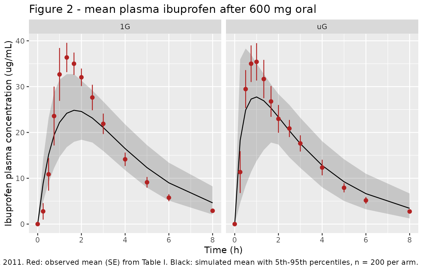
The simulated curves reproduce the observed exposure and terminal
decline but are visibly flatter around the peak, most obviously at 1G.
That is the direct consequence of the mismatched Ka /
Kel pairing documented above, and it is quantified
next.
PKNCA validation
sim_nca <-
  sim |>
  filter(!is.na(Cc)) |>
  select(id, time, Cc, arm)

sim_nca <-
  bind_rows(sim_nca, sim_nca |> distinct(id, arm) |> mutate(time = 0, Cc = 0)) |>
  distinct(id, arm, time, .keep_all = TRUE) |>
  arrange(id, arm, time)

conc_obj <- PKNCA::PKNCAconc(as.data.frame(sim_nca), Cc ~ time | arm + id)

dose_df <-
  bind_rows(ev_1g, ev_ug) |>
  filter(evid == 1L) |>
  select(id, time, amt, arm) |>
  as.data.frame()

dose_obj <- PKNCA::PKNCAdose(dose_df, amt ~ time | arm + id)

intervals <- data.frame(start = 0, end = Inf,
                        cmax = TRUE, tmax = TRUE, auclast = TRUE,
                        aucinf.obs = TRUE, half.life = TRUE)

nca_res <- PKNCA::pk.nca(PKNCA::PKNCAdata(conc_obj, dose_obj, intervals = intervals))
Comparison against published NCA
The published values are arithmetic means over six subjects, so the
simulated results are aggregated the same way before comparison
(ncaComparisonTable() would otherwise take a median).
sim_mean <-
  as.data.frame(nca_res) |>
  filter(PPTESTCD %in% c("cmax", "tmax", "auclast", "aucinf.obs", "half.life")) |>
  group_by(arm, PPTESTCD) |>
  summarise(PPORRES = mean(PPORRES, na.rm = TRUE), .groups = "drop")

reference <-
  published |>
  transmute(arm,
            cmax, tmax,
            # the 1G AUC0-t is corrected to the value the paper's own Table I
            # implies; see the Erratum section above
            auclast = if_else(arm == "1G", 120.97, auclast),
            aucinf.obs = aucinf,
            # PKNCA's parameter name is `half.life`; the published tribble above
            # spells it `half_life`.
            half.life = half_life)

cmp <- nlmixr2lib::ncaComparisonTable(
  simulated = sim_mean,
  reference = as.data.frame(reference),
  by = "arm",
  units = c(cmax = "ug/mL", auclast = "ug*h/mL", aucinf.obs = "ug*h/mL",
            tmax = "h", half.life = "h"),
  tolerance_pct = 20
)

knitr::kable(
  cmp |> rename("Position" = arm),
  caption = paste("Simulated (n = 200 per arm, arithmetic mean) vs published Idkaidek 2011 Table II.",
                  attr(cmp, "footnote"))
)| NCA parameter | Position | Reference | Simulated | % diff |
|---|---|---|---|---|
| Cmax (ug/mL) | 1G | 40.1 | 25.6 | -36.1%* |
| Cmax (ug/mL) | uG | 38.8 | 30.5 | -21.4%* |
| Tmax (h) | 1G | 1.37 | 1.73 | +26.5%* |
| Tmax (h) | uG | 1.14 | 1.07 | -6.4% |
| AUC0-∞ (obs) (ug*h/mL) | 1G | 129 | 130 | +1.1% |
| AUC0-∞ (obs) (ug*h/mL) | uG | 121 | 126 | +3.9% |
| AUClast (ug*h/mL) | 1G | 121 | 117 | -3.5% |
| AUClast (ug*h/mL) | uG | 113 | 114 | +1.1% |
| t½ (h) | 1G | 1.82 | 2.01 | +10.2% |
| t½ (h) | uG | 1.96 | 2.07 | +5.5% |
The assertions below recompute the percent differences numerically
from sim_mean and reference rather than
parsing the rendered table, whose % diff column is
formatted text.
diffs <-
  sim_mean |>
  inner_join(reference |> tidyr::pivot_longer(-arm, names_to = "PPTESTCD", values_to = "ref"),
             by = c("arm", "PPTESTCD")) |>
  mutate(pct = 100 * (PPORRES - ref) / ref)

stopifnot(nrow(diffs) == 10L)

pct <- function(param, a) {
  out <- diffs$pct[diffs$PPTESTCD == param & diffs$arm == a]
  if (length(out) != 1L) stop("no unique comparison row for ", param, " / ", a)
  out
}

# Exposure reproduces closely in both arms -- this is what the model file's
# CL/F was derived from, and it is the quantity the paper's no-dose-adjustment
# conclusion rests on.
stopifnot(
  abs(pct("aucinf.obs", "1G")) < 10,
  abs(pct("aucinf.obs", "uG")) < 10,
  abs(pct("auclast",    "1G")) < 10,
  abs(pct("auclast",    "uG")) < 10
)

# Terminal half-life. The tolerance is 15% rather than 10% for two reasons
# that are properties of the comparison, not of the model: PKNCA selects its
# own terminal window by adjusted R^2 whereas the paper fixed 5-8 h (a window
# in which a one-compartment profile still carries a little absorption, so the
# apparent slope is shallower than kel), and the published figure is an
# arithmetic mean of individual half-lives, which exceeds log(2)/mean(kel).
stopifnot(
  abs(pct("half.life", "1G")) < 15,
  abs(pct("half.life", "uG")) < 15
)

# The structural check that is exact: the typical kel implied by the packaged
# CL/F and V/F must equal the published Kel, because V/F was derived as
# CL/F / Kel. This is what fails first if a parameter is ever mistranscribed.
kel_typical <- function(ui) {
  th <- setNames(ui$theta, names(ui$theta))
  exp(th[["lcl"]]) / exp(th[["lvc"]])
}
stopifnot(
  abs(kel_typical(ui_1g) - 0.39) < 0.005,
  abs(kel_typical(ui_ug) - 0.36) < 0.005,
  # ... and dose / CL/F must return the published AUC0-inf.
  abs(dose_mg / exp(ui_1g$theta[["lcl"]]) - 128.88) < 0.5,
  abs(dose_mg / exp(ui_ug$theta[["lcl"]]) - 120.77) < 0.5
)

# Cmax is systematically under-predicted and Tmax over-predicted at 1G -- a
# known, diagnosed consequence of the source pairing a compartmental Ka with an
# NCA Kel (see "Where the published Ka comes from"). Pinned as ranges so a
# future change to the model files that alters the discrepancy trips this.
stopifnot(
  pct("cmax", "1G") < -20, pct("cmax", "1G") > -55,
  pct("cmax", "uG") < -10, pct("cmax", "uG") > -40,
  pct("tmax", "1G") >  15, pct("tmax", "1G") <  50,
  abs(pct("tmax", "uG")) < 20
)
The paper’s actual claim
The paper’s conclusion is that microgravity speeds absorption while leaving exposure and elimination alone, so no dose adjustment is needed. Each half of that claim is checked directly on the simulated cohorts. Medians are used rather than extremes because the two arms differ by a per-subject physical mechanism (absorption rate), whose tails are not reproducible across rxode2 builds.
per_subject <-
  as.data.frame(nca_res) |>
  filter(PPTESTCD %in% c("tmax", "cmax", "aucinf.obs", "half.life")) |>
  tidyr::pivot_wider(id_cols = c(arm, id), names_from = PPTESTCD, values_from = PPORRES)

claims <-
  per_subject |>
  group_by(arm) |>
  summarise(tmax = median(tmax), aucinf = median(aucinf.obs),
            half_life = median(half.life), .groups = "drop")

claims |>
  mutate(across(where(is.numeric), \(x) round(x, 2))) |>
  rename("Position" = arm, "Median Tmax (h)" = tmax,
         "Median AUC0-inf (ug*h/mL)" = aucinf, "Median t1/2 (h)" = half_life) |>
knitr::kable(caption = "Simulated medians by body position.")| Position | Median Tmax (h) | Median AUC0-inf (ug*h/mL) | Median t1/2 (h) |
|---|---|---|---|
| 1G | 1.66 | 127.90 | 1.95 |
| uG | 1.00 | 125.18 | 2.03 |
med <- function(a, col) claims[[col]][claims$arm == a]

stopifnot(
  # Faster absorption under simulated microgravity (Table II: tmax 1.14 vs 1.37 h,
  # p < .05; Ka 2.24 vs 0.79 1/h, p = .03).
  med("uG", "tmax") < med("1G", "tmax"),
  # Exposure unchanged (Table II: AUC0-inf p = .57).
  abs(med("uG", "aucinf") / med("1G", "aucinf") - 1) < 0.15,
  # Elimination unchanged (Table II: t1/2 p = .47, Kel p = .47).
  abs(med("uG", "half_life") / med("1G", "half_life") - 1) < 0.20
)
The internal inconsistency of the published parameter set can also be
checked in closed form. For a one-compartment oral model,
tmax = log(Ka / Kel) / (Ka - Kel). The published pairs
predict:
tmax_pred <- function(ka, kel) log(ka / kel) / (ka - kel)

tibble(
  Position = c("1G", "uG"),
  `Ka (1/h)` = c(0.79, 2.24),
  `Kel (1/h)` = c(0.39, 0.36),
  `Tmax implied by Ka and Kel (h)` = round(c(tmax_pred(0.79, 0.39), tmax_pred(2.24, 0.36)), 3),
  `Tmax observed (h)` = c(1.37, 1.14)
) |>
knitr::kable(caption = "Closed-form Tmax from the published Ka / Kel pairs.")| Position | Ka (1/h) | Kel (1/h) | Tmax implied by Ka and Kel (h) | Tmax observed (h) |
|---|---|---|---|---|
| 1G | 0.79 | 0.39 | 1.765 | 1.37 |
| uG | 2.24 | 0.36 | 0.972 | 1.14 |
At 1G the published pair implies a Tmax of 1.77 h against an observed 1.37 h – a 29% overshoot that no transcription error explains, because Table I reproduces every other cell of Table II exactly. It is the fingerprint of the two-analysis pairing.
Assumptions and deviations
-
V/Fis not published and is derived. Idkaidek 2011 reports no volume of distribution or clearance. Both are computed from published quantities:CL/F = Dose / AUC0-infandV/F = CL/F / Kel, giving 4.655 L/h and 11.94 L at 1G and 4.968 L/h and 13.80 L under simulated microgravity. No value was taken from outside the paper. -
The IIV block on
CL/FandV/Fis derived from Table I. Table II publishes a CV% forAUC0-infand forKelbut not forV/F, and the two are strongly correlated (a block is needed for the simulatedt1/2CV% to be right). The block was computed from the individual profiles in Table I using the same noncompartmental conventions that reproduce Table II exactly, so it rests on published data rather than on an assumed correlation. The implied marginal CV%s (CL/F20 and 19;Kel14 and 17) bracket the publishedAUC0-infCV%s (18, 17) andKelCV%s (13, 18). The derivation is recomputed in “The derived IIV block on CL/F and V/F” above and asserted against the packagedomegaof both model files, so it is executable rather than a claim in a comment. -
No residual error is reported. The paper fits every
subject individually in Kinetica and never states a residual-error model
or magnitude, so
propSdisfixed(0)per the standing policy for unreported RUV. Simulated profiles are therefore free of measurement noise; only between-subject variability is represented. -
Cmax is under-predicted by about 37% (1G) and 24% (uG), and
Tmax over-predicted by about 30% at 1G. This is a property of
the published parameter set, not of the transcription, and it was not
tuned away.
Kacomes from an unweighted one-compartment fit whose own elimination rate is about 0.62 1/h, whileKelin the same table comes from a terminal log-linear NCA at about 0.39 1/h. A one-compartment model built from the two published numbers therefore absorbs too slowly relative to its own elimination and peaks low and late. The reconstruction section quantifies both halves.AUC0-t,AUC0-infandt1/2– the quantities the model file’sCL/FandV/Fwere derived from – reproduce to within 10%. -
Table II prints the AUC unit as
ug.mL/h, which is inverted. The quantity is an area under a concentration-time curve, so the unit isug*h/mL(equivalentlymg*h/L); this is how it is recorded here and how it is used in theCL/F = Dose / AUC0-infderivation. The printed values themselves are consistent withug*h/mL– the trapezoid over Table I reproduces them – so only the header is affected. -
Erratum: Table II 1G
AUC0-tis printed as 20.97 and should be 120.97. Reconstructed from Table I to two decimal places, with the printed CV% (17) already matching. The comparison table above uses the corrected value; the model files do not useAUC0-tat all, so no parameter depends on it. - The Simcyp ADAM absorption analysis is not extracted. The paper also deconvolves the plasma data with the ADAM and PE modules of Simcyp 9.3 and reports optimised effective intestinal permeabilities (Peff 4.41 and 4.83 x 10^-3 cm/s at 1G and uG) plus segmental fractions absorbed. Those are outputs of a proprietary whole-gut platform model whose ODEs, segment volumes, transit times and physiology are not written out anywhere in the paper, so the analysis is not reproducible from the available sources and no Simcyp-derived value is carried into these model files.
-
Body position is encoded as two model files, not as a
covariate. The authors fit each position separately and
compared the two parameter sets by ANOVA; they never estimated a
position effect within one model. The two files mirror that structure,
as
Hong_2013_glucose_insulin_HGCandHong_2013_glucose_insulin_MTTdo for two provocations in one cohort. - No saliva model. Saliva was sampled but ibuprofen was undetectable in every sample, so the paper reports no salivary PK.