Elranatamab population PK and CRS exposure-response (Hibma 2026)
Source:vignettes/articles/Hibma_2026_elranatamab.Rmd
Hibma_2026_elranatamab.RmdModel and source
Hibma 2026 contributes two models, both documented in this article:
-
Hibma_2026_elranatamab– the population PK model. It is a two-compartment semi-mechanistic target-binding model for free and total elranatamab and free and total soluble BCMA (sBCMA). -
Hibma_2026_elranatamab_crs– the landmark logistic exposure-response model for any-grade cytokine release syndrome (CRS) after the first step-up priming dose. Its exposure input is the Day 4 free elranatamab trough, which comes from the PK model.
mod_pk <- readModelDb("Hibma_2026_elranatamab")
mod_crs <- readModelDb("Hibma_2026_elranatamab_crs")
ui_pk <- rxode2::rxode(mod_pk)
#> ℹ parameter labels from comments will be replaced by 'label()'
ui_crs <- rxode2::rxode(mod_crs)- Citation: Hibma JE, Irby D, Liu A, Elmeliegy M, King LE, Gifondorwa D, Jiang S, Poels KE, Soltantabar P, Lon H-K, Shtylla B, Wang D, Williams JH, Nicholas T. Elranatamab population pharmacokinetics and exposure-response for cytokine release syndrome in patients with relapsed or refractory multiple myeloma. Clin Pharmacokinet. 2026;65:1173-1192. doi:10.1007/s40262-026-01663-z.
- Description (PK): Two-compartment semi-mechanistic target-binding population PK model for the BCMA x CD3 bispecific antibody elranatamab in adults with relapsed or refractory multiple myeloma (Hibma 2026; MagnetisMM-1, -2, -3 and -9, N = 321). Elranatamab binds soluble BCMA (sBCMA) in the central compartment under rapid (quasi-)equilibrium with dissociation constant Kd; free drug, free sBCMA and the elranatamab-sBCMA complex each carry their own clearance and volume. States are total elranatamab (free + complex) in the central compartment, free elranatamab in the peripheral compartment, and total sBCMA with zero-order synthesis; the complex amount is the closed-form root of the binding quadratic. SC absorption is first order with bioavailability F; IV doses are 1-h infusions. Covariates: sex on elranatamab CL (linear), baseline body weight on elranatamab Vc and age on ka (power). Outputs: free (Cc) and total (Cc_total) elranatamab in ng/mL, free (Ctarget) and total (Ctotal_target) sBCMA in nM, each with proportional residual error. The companion landmark exposure-response model for cytokine release syndrome is Hibma_2026_elranatamab_crs.
- Description (CRS): Binomial logistic-regression exposure-safety model for any-grade cytokine release syndrome (CRS) after the FIRST step-up priming dose (12 mg SC on Cycle 1 Day 1) of the BCMA x CD3 bispecific antibody elranatamab in adults with relapsed or refractory multiple myeloma (Hibma 2026; MagnetisMM-3, N = 183, 79 events). The probability of CRS is expit(-7.65 + 1.14 * TUM_BURDEN_HIGH + 1.35 * log(CTROUGH)), where CTROUGH is the individual FREE elranatamab trough concentration in ng/mL on Day 4, just before the second (32 mg) step-up dose, and TUM_BURDEN_HIGH flags high baseline tumour burden (ESM Table S2). The log is natural (odds ratio 3.86 = exp(1.35) per unit of log(Ctrough)). There is no PK layer and no ODE: the exposure is supplied as a data column, derived in the source from post-hoc estimates of the companion population PK model Hibma_2026_elranatamab. No random effect and no residual error are estimated (Bernoulli likelihood). No exposure-response relationship was significant after the second step-up dose, and none could be fitted after the first full dose, so this is the paper’s only CRS model.
- Article: https://doi.org/10.1007/s40262-026-01663-z (open access, PMC13461831)
The CRS model’s parameters are printed in electronic supplementary material (ESM) Table S2. The PK equations and Table 2 are in the main text.
Elranatamab is a BCMA x CD3 bispecific antibody. A mechanistic QSP
model of the same drug, fitted to the same MagnetisMM-1 and -3
programme, is available as Poels_2025_elranatamab_qsp.
Population
The PK model was fitted to 321 adults with relapsed or refractory multiple myeloma from four studies (Hibma 2026 Table 1, ESM Table S1):
- MagnetisMM-1: IV (1-h infusion) and SC dose escalation, step-up regimens and fixed-dose expansion; n = 87.
- MagnetisMM-2: Japanese patients; n = 4.
- MagnetisMM-3 Cohorts A and B: 12/32/76 mg step-up, then 76 mg QW; n = 187.
- MagnetisMM-9: 4/20/76 mg step-up; n = 43.
Doses ranged from 0.1 to 1000 ug/kg, and fixed doses from 4 to 76 mg. The data were 13,233 observations: 3739 total elranatamab, 2947 free elranatamab, 3812 total sBCMA and 2735 free sBCMA.
The cohort was 48% female (154/321), 60% White, 15% Asian, 9% Black and 16% race missing. Median age was 66 years (range 36-89) and median body weight 71.5 kg (36.5-159.6). Median baseline sBCMA was 8.29 nM (0.00-266.67).
The CRS analysis used the 183 MagnetisMM-3 participants who received the two step-up priming doses. There were 79 any-grade CRS events (43%) after the first step-up dose, 35 (19%) after the second and 13 (7%) after the first full dose. Baseline tumour burden in this population was low or intermediate in 131 (72%), high in 38 (21%) and missing in 14 (7.7%).
str(ui_pk$population)
#> List of 13
#>  $ species       : chr "human"
#>  $ n_subjects    : int 321
#>  $ n_studies     : int 4
#>  $ n_observations: chr "13,233 non-BLQ observations: 3739 total elranatamab, 2947 free elranatamab, 3812 total sBCMA, 2735 free sBCMA ("| __truncated__
#>  $ age_range     : chr "36-89 years (median 66)"
#>  $ weight_range  : chr "36.5-159.6 kg (median 71.5)"
#>  $ sex_female_pct: num 48
#>  $ race_ethnicity: Named num [1:4] 60 15 9 16
#>   ..- attr(*, "names")= chr [1:4] "White" "Asian" "Black" "Missing"
#>  $ disease_state : chr "Relapsed or refractory multiple myeloma"
#>  $ dose_range    : chr "IV (1-h infusion) 0.1-50 ug/kg QW and SC 80-1000 ug/kg QW (MagnetisMM-1 Part 1); SC 600 then 1000 ug/kg QW or Q"| __truncated__
#>  $ regions       : chr "Multinational (MagnetisMM-2 enrolled Japanese patients only)"
#>  $ baseline_sbcma: chr "median 8.29 nM, range 0.00-266.67 (Table 1)"
#>  $ notes         : chr "MagnetisMM-1 (NCT03269136) Parts 1, 1.1 and 2A (n = 53 + 19 + 15), MagnetisMM-2 (NCT04798586, n = 4), MagnetisM"| __truncated__
str(ui_crs$population)
#> List of 11
#>  $ species       : chr "human"
#>  $ n_subjects    : int 183
#>  $ n_studies     : int 1
#>  $ n_observations: chr "183 binary any-grade CRS outcomes after the first step-up priming dose (79 events, 43%; 104 non-events)"
#>  $ age_range     : chr "36-89 years (MagnetisMM-3 Cohorts A and B; medians 68 and 67; Table 1)"
#>  $ weight_range  : chr "36.5-159.6 kg (MagnetisMM-3 Cohorts A and B; medians 72.0 and 69.3; Table 1)"
#>  $ disease_state : chr "Relapsed or refractory multiple myeloma"
#>  $ dose_range    : chr "SC elranatamab 12 mg on C1D1, 32 mg on C1D4, 76 mg on C1D8 then 76 mg QW (two-step-up priming regimen)"
#>  $ regions       : chr "Multinational (MagnetisMM-3, NCT04649359)"
#>  $ tumor_burden  : chr "MagnetisMM-3 exposure-response population: low or intermediate 131 (72%), high 38 (21%), missing 14 (7.7%) (Table 1)"
#>  $ notes         : chr "Data cutoff March 2024. After the second step-up dose 35 CRS events (19%) occurred with no significant exposure"| __truncated__
Source trace
| Equation / parameter | Value | Source location |
|---|---|---|
d/dt(central) (A1, total drug) |
ka*A3 - k12*(A1 - X) + k21*A2 - CL*Cf - CLcomplex*Ccomplex |
Section 2.4, equation for dA1/dt |
d/dt(peripheral1) (A2) |
k12*(A1 - X) - k21*A2 |
Section 2.4, dA2/dt |
d/dt(depot) (A3) |
-ka*A3 |
Section 2.4, dA3/dt |
d/dt(total_target) (A4, total sBCMA) |
ksyn - CLsBCMA*Cf,sBCMA - CLcomplex*Ccomplex |
Section 2.4, dA4/dt |
| Free / complex concentrations |
Cf = (A1-X)/Vc;
Cf,sBCMA = (A4-X)/Vc,sBCMA;
Ccomplex = X/Vc,complex
|
Section 2.4 |
Complex amount X
|
smaller root of the Kd quadratic, rationalised | Section 2.4, Xcomplex equation |
| Total concentrations |
Ct = Cf + Ccomplex (drug and sBCMA) |
Section 2.4 |
ksyn, total_target(0)
|
CLsBCMA * BLsBCMA; BLsBCMA * Vc,sBCMA
|
Not printed; drug-free steady state (see Assumptions) |
| Molecular weight | 148 kDa (sBCMA 5.4 kDa) | Section 2.2 |
lcl |
log(0.324) L/day | Table 2; Section 3.3 equation |
e_sexf_cl |
-0.492 (linear, female) | Table 2; Section 3.3 equation |
lvc |
log(4.777) L | Table 2 |
e_wt_vc |
1.017, reference 71.45 kg | Table 2; Section 3.3 equation |
lvp, lq
|
log(2.83) L, log(0.225) L/day | Table 2 |
lka |
log(0.287) 1/day | Table 2 |
e_age_ka |
-1.459, reference 66 years | Table 2; Section 3.3 equation |
lfdepot |
log(0.562) | Table 2 |
lcl_target, lvc_target
|
log(0.273) L/day, log(15.418) L | Table 2 |
lrbase_target |
log(6.914) nM | Table 2 (BLsBCMA) |
lcl_complex, lvc_complex
|
log(0.164) L/day, log(3.802) L | Table 2 |
lkd |
log(3.138) nM | Table 2 |
| IIV variances |
(CV/100)^2 of the Table 2 ‘CV (%)’ column |
Table 2 (scale verified below) |
| Residual SDs | free drug 0.347, total drug 0.422, free sBCMA 0.518, total sBCMA 0.347 | Table 2 |
logit_ref (CRS) |
-7.65 | ESM Table S2 |
e_tum_burden_high_logit |
1.14 (OR 3.11) | ESM Table S2 |
e_ctrough_logit |
1.35 (OR 3.86) per unit of natural log(Ctrough, ng/mL) | ESM Table S2 |
IIV scale: CV% = 100 * sqrt(omega^2)
Table 2 reports each IIV as a “CV (%)” with an RSE and a 95% CI. The
printed CI is reproduced exactly by a symmetric Wald interval on
omega^2, with the RSE on the variance scale, mapped back
through sqrt(). The exact log-normal CV,
sqrt(exp(omega^2) - 1), does not reproduce the CIs. The
variances in the model are therefore (CV/100)^2. This
matters a lot here: for CLsBCMA (448% CV) the two readings give
omega^2 = 20.1 and 3.05.
tab2 <- tibble::tribble(
  ~parameter,   ~cv,    ~rse,   ~lo,    ~hi,
  "Vc",         68.56,  13.346, 58.91,  77.01,
  "Vc,sBCMA",   135.98, 31.91,  83.25,  173.38,
  "CLsBCMA",    448.07, 15.702, 372.8,  512.41,
  "CLcomplex",  79.18,  19.338, 62.45,  93.01,
  "Vc,complex", 70.07,  17.261, 57.01,  81.06,
  "BLsBCMA",    134.61, 13.078, 116.1,  150.9,
  "ka",         68.41,  14.538, 57.88,  77.59
)
iiv_chk <- tab2 |>
  mutate(
    omega2 = (cv / 100)^2,
    se = rse / 100 * omega2,
    lo_sqrt = 100 * sqrt(omega2 - 1.96 * se),
    hi_sqrt = 100 * sqrt(omega2 + 1.96 * se),
    # Alternative reading: exact log-normal CV
    omega2_ln = log(1 + (cv / 100)^2),
    hi_ln = 100 * sqrt(exp(omega2_ln + 1.96 * rse / 100 * omega2_ln) - 1)
  )
iiv_chk |>
  select(parameter, cv, lo, lo_sqrt, hi, hi_sqrt, hi_ln) |>
  rename(
    "Parameter" = parameter, "CV (%)" = cv,
    "Printed lower" = lo, "sqrt-reading lower" = lo_sqrt,
    "Printed upper" = hi, "sqrt-reading upper" = hi_sqrt,
    "log-normal-reading upper" = hi_ln
  ) |>
knitr::kable(digits = 2, caption = "Table 2 IIV confidence intervals under two readings of 'CV (%)'.")| Parameter | CV (%) | Printed lower | sqrt-reading lower | Printed upper | sqrt-reading upper | log-normal-reading upper |
|---|---|---|---|---|---|---|
| Vc | 68.56 | 58.91 | 58.91 | 77.01 | 77.01 | 79.12 |
| Vc,sBCMA | 135.98 | 83.25 | 83.22 | 173.38 | 173.36 | 211.75 |
| CLsBCMA | 448.07 | 372.80 | 372.80 | 512.41 | 512.40 | 727.00 |
| CLcomplex | 79.18 | 62.45 | 62.40 | 93.01 | 92.98 | 97.80 |
| Vc,complex | 70.07 | 57.01 | 57.00 | 81.06 | 81.06 | 84.07 |
| BLsBCMA | 134.61 | 116.10 | 116.08 | 150.90 | 150.88 | 163.26 |
| ka | 68.41 | 57.88 | 57.85 | 77.59 | 77.55 | 79.86 |
# Deterministic: the sqrt reading reproduces every printed bound to within
# 0.05 CV points; the log-normal reading overshoots every upper bound, by
# 2.1-4.8 points for the moderate CVs and by 38 and 215 points for Vc,sBCMA
# and CLsBCMA.
stopifnot(
  max(abs(iiv_chk$lo_sqrt - iiv_chk$lo)) < 0.2,
  max(abs(iiv_chk$hi_sqrt - iiv_chk$hi)) < 0.2,
  all(iiv_chk$hi_ln - iiv_chk$hi > 1.5),
  max(iiv_chk$hi_ln - iiv_chk$hi) > 100
)

# The packaged variances equal (CV/100)^2.
om <- diag(ui_pk$omega)
stopifnot(
  abs(om[["etalcl_target"]] - 4.4807^2) < 1e-4,
  abs(om[["etalvc"]] - 0.6856^2) < 1e-4,
  abs(om[["etalrbase_target"]] - 1.3461^2) < 1e-4
)
CRS odds ratios
The CRS model’s printed odds ratios should equal the exponentiated estimates. With two-decimal rounding on both columns the test is an interval one: there must be a coefficient that rounds to the printed estimate and whose exponential rounds to the printed odds ratio.
or_consistent <- function(est, or, digits = 2) {
  b <- seq(est - 0.5 * 10^-digits, est + 0.5 * 10^-digits, length.out = 2001)
  any(round(b, digits) == est & round(exp(b), digits) == or)
}
ini_crs <- ui_crs$theta
stopifnot(
  or_consistent(ini_crs[["e_ctrough_logit"]], 3.86),
  or_consistent(ini_crs[["e_tum_burden_high_logit"]], 3.11),
  # 95% CI of the odds ratios equal exp() of the coefficient CIs
  abs(exp(0.869) - 2.38) < 0.01, abs(exp(1.88) - 6.55) < 0.01,
  abs(exp(0.335) - 1.40) < 0.01, abs(exp(1.97) - 7.17) < 0.01
)
Typical-value checks
The helper below builds an event table. Observation rows carry
dvid = 1 and no cmt, because the model has
four observed outputs and none of them is an ODE state. Every output
column (Cc, Cc_total, Ctarget,
Ctotal_target) is returned at every observation row.
make_events <- function(ids, dose_times, dose_amts, obs_times,
                        route = c("sc", "iv"), inf_dur = 1 / 24) {
  route <- match.arg(route)
  dose <- tidyr::expand_grid(id = ids, k = seq_along(dose_times)) |>
    mutate(
      time = dose_times[k], amt = dose_amts[k], evid = 1L,
      cmt = if (route == "sc") "depot" else "central",
      rate = if (route == "sc") 0 else amt / inf_dur,
      dvid = NA_integer_
    ) |>
    select(-k)
  obs <- tidyr::expand_grid(id = ids, time = obs_times) |>
    mutate(amt = 0, evid = 0L, cmt = NA_character_, rate = 0, dvid = 1L)
  bind_rows(dose, obs) |> arrange(id, time, desc(evid))
}
typical_covs <- function(ev, SEXF = 0, WT = 71.45, AGE = 66) {
  ev$SEXF <- SEXF
  ev$WT <- WT
  ev$AGE <- AGE
  ev
}
mod_typ <- rxode2::zeroRe(ui_pk)
solve_typ <- function(ev, model = mod_typ) {
  as.data.frame(rxode2::rxSolve(model, events = ev, returnType = "data.frame",
                                useLinCmt = FALSE))
}
Derived rate constants and half-life
The Discussion quotes elimination rate constants of 0.068/day for free drug (CL/Vc) and 0.043/day for the complex (CLcomplex/Vc,complex). It also gives a half-life of about 22 days at 76 mg. The first two follow directly from Table 2. For the half-life, a typical male receives 76 mg QW for 24 weeks and the terminal slopes of total and free elranatamab are fitted between 60 and 120 days after the last dose. The paper does not say which analyte its 22-day half-life refers to. Total elranatamab matches it. Free drug declines faster (about 18 days) because the bound fraction grows as concentrations fall towards the sBCMA pool.
th <- ui_pk$theta
kel_free <- exp(th[["lcl"]]) / exp(th[["lvc"]])
kel_complex <- exp(th[["lcl_complex"]]) / exp(th[["lvc_complex"]])

ev_hl <- make_events(1L, c(seq(0, 161, 7)), rep(76, 24), seq(0, 400, 1)) |>
  typical_covs()
s_hl <- solve_typ(ev_hl)
#> ℹ omega/sigma items treated as zero: 'etalcl', 'etalvc', 'etalvp', 'etalq', 'etalka', 'etalfdepot', 'etalcl_target', 'etalvc_target', 'etalrbase_target', 'etalcl_complex', 'etalvc_complex', 'etalkd'
term <- s_hl |> filter(time >= 161 + 60, time <= 161 + 120)
t_half <- log(2) / -coef(lm(log(Cc_total) ~ time, data = term))[["time"]]
t_half_free <- log(2) / -coef(lm(log(Cc) ~ time, data = term))[["time"]]

tibble::tibble(
  quantity = c("kel, free elranatamab (1/day)", "kel, complex (1/day)",
               "terminal half-life, total (day)", "terminal half-life, free (day)"),
  model = c(kel_free, kel_complex, t_half, t_half_free),
  paper = c(0.068, 0.043, 22, NA)
) |>
  rename("Quantity" = quantity, "Model" = model, "Hibma 2026" = paper) |>
knitr::kable(digits = 3)| Quantity | Model | Hibma 2026 |
|---|---|---|
| kel, free elranatamab (1/day) | 0.068 | 0.068 |
| kel, complex (1/day) | 0.043 | 0.043 |
| terminal half-life, total (day) | 22.023 | 22.000 |
| terminal half-life, free (day) | 17.818 | NA |
Drug-free steady state of sBCMA
With no drug the sBCMA synthesis and elimination balance at the estimated baseline, so free and total sBCMA stay at 6.914 nM.
ev_ss <- make_events(1L, 0, 0, seq(0, 200, 10)) |> typical_covs()
s_ss <- solve_typ(ev_ss)
#> ℹ omega/sigma items treated as zero: 'etalcl', 'etalvc', 'etalvp', 'etalq', 'etalka', 'etalfdepot', 'etalcl_target', 'etalvc_target', 'etalrbase_target', 'etalcl_complex', 'etalvc_complex', 'etalkd'
stopifnot(
  max(abs(s_ss$Ctarget / 6.914 - 1)) < 1e-6,
  max(abs(s_ss$Ctotal_target / 6.914 - 1)) < 1e-6,
  max(abs(s_ss$Cc)) < 1e-8
)
IV route: target binding at low doses
The IV path is exercised with 1-h infusions at two MagnetisMM-1 Part
1 dose levels, for a 71.45 kg typical male. Even 50 ug/kg (3.6 mg) gives
only about 5 nM of drug, less than the ~7 nM sBCMA pool. At every IV
dose free drug is therefore close to its analytic low-dose fraction of
total, Kd / (Kd + BLsBCMA) = 0.31. At 76 mg SC steady state
the drug exceeds the pool by more than 10-fold, and free and total
converge.
iv <- bind_rows(lapply(c(1, 50), function(ugkg) {
  amt <- ugkg * 71.45 / 1000
  make_events(1L, 0, amt, c(seq(0, 1, 1 / 24), seq(1.5, 28, 0.5)), route = "iv") |>
    typical_covs() |>
    solve_typ() |>
    mutate(dose = paste(ugkg, "ug/kg IV"))
}))
#> ℹ omega/sigma items treated as zero: 'etalcl', 'etalvc', 'etalvp', 'etalq', 'etalka', 'etalfdepot', 'etalcl_target', 'etalvc_target', 'etalrbase_target', 'etalcl_complex', 'etalvc_complex', 'etalkd'
#> ℹ omega/sigma items treated as zero: 'etalcl', 'etalvc', 'etalvp', 'etalq', 'etalka', 'etalfdepot', 'etalcl_target', 'etalvc_target', 'etalrbase_target', 'etalcl_complex', 'etalvc_complex', 'etalkd'
iv |>
  select(time, dose, Free = Cc, Total = Cc_total) |>
  pivot_longer(c(Free, Total), names_to = "analyte", values_to = "conc") |>
  filter(conc > 0) |>
  ggplot(aes(time, conc, colour = analyte)) +
  geom_line() +
  facet_wrap(~dose, scales = "free_y") +
  scale_y_log10() +
  labs(x = "Time (day)", y = "Elranatamab (ng/mL)", colour = NULL,
       title = "Typical-value IV profiles, free vs total elranatamab")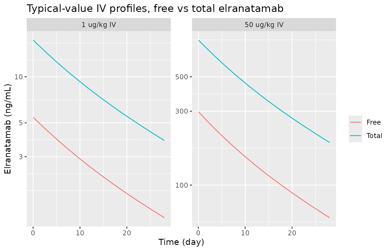
frac_free <- iv |>
  filter(time == 1) |>
  mutate(f = Cc / Cc_total) |>
  pull(f, name = dose)
frac_limit <- exp(th[["lkd"]]) / (exp(th[["lkd"]]) + exp(th[["lrbase_target"]]))
frac_ss <- s_hl$Cc[s_hl$time == 161] / s_hl$Cc_total[s_hl$time == 161]
c(frac_limit = frac_limit, frac_free, frac_76mg_ss = frac_ss)
#>   frac_limit   1 ug/kg IV  50 ug/kg IV frac_76mg_ss
#>    0.3121767    0.3127711    0.3430444    0.9108057
# Deterministic: 1 ug/kg sits within 0.01 of the analytic limit; 76 mg QW
# steady state is > 85% free (typical value 0.91).
stopifnot(
  abs(frac_free[["1 ug/kg IV"]] - frac_limit) < 0.01,
  frac_free[["50 ug/kg IV"]] < 0.45,
  frac_ss > 0.85
)
Virtual cohort
The observed data are not public. The virtual patients draw covariates to match the pooled analysis population in Table 1: 48% female; body weight log-normal with median 71.5 kg and CV 24%, truncated to 36.5-159.6 kg; age normal with mean 65.3 years and SD 9.7, truncated to 36-89 years. Random effects are drawn from the model’s OMEGA. Each scenario gets its own 150 virtual patients.
# rxode2 random streams are partitioned per solver thread, so the cohort
# below differs between machines with different thread counts; every
# assertion downstream is written to hold for any cohort (robust medians and
# geometric means with generous headroom, never extremes).
set.seed(20260929)
rxode2::rxSetSeed(20260929)
draw_covs <- function(n) {
  tibble::tibble(
    SEXF = rbinom(n, 1, 0.48),
    WT = pmin(pmax(71.5 * exp(rnorm(n, 0, 0.24)), 36.5), 159.6),
    AGE = pmin(pmax(round(rnorm(n, 65.3, 9.7)), 36), 89)
  )
}
n_per <- 150L

# Approved regimen: 12 mg on Day 1, 32 mg on Day 4, 76 mg QW from Day 8.
# Responders move to Q2W after week 24 (Day 169) and Q4W after week 48
# (Day 337). Time 0 is Day 1.
qw <- seq(7, 161, 7)
q2w <- seq(168, 322, 14)
q4w <- seq(336, 476, 28)
scen <- list(
  "S1: last 76 mg on C1D8" = c(0, 3, 7),
  "S2: last 76 mg on C1D15" = c(0, 3, 7, 14),
  "S3: last 76 mg on C2D1" = c(0, 3, 7, 14, 21, 28),
  "S4: QW to week 24" = c(0, 3, qw),
  "S5: + Q2W to week 48" = c(0, 3, qw, q2w),
  "S6: + Q4W to week 72" = c(0, 3, qw, q2w, q4w)
)
events <- bind_rows(lapply(seq_along(scen), function(i) {
  dt <- scen[[i]]
  last <- max(dt)
  obs <- sort(unique(c(seq(0, last + 200, 1), 3)))
  ids <- (i - 1L) * n_per + seq_len(n_per)
  make_events(ids, dt, c(12, 32, rep(76, length(dt) - 2)), obs) |>
    left_join(draw_covs(n_per) |> mutate(id = ids), by = "id") |>
    mutate(scenario = names(scen)[i], last_dose = last,
           n76 = length(dt) - 2L)
}))
stopifnot(!anyDuplicated(unique(events[, c("id", "time", "evid")])))
Simulation
sim <- rxode2::rxSolve(
  mod_pk, events = events,
  keep = c("scenario", "last_dose", "n76", "SEXF", "WT", "AGE"),
  returnType = "data.frame", useLinCmt = FALSE
) |>
  as.data.frame()
#> ℹ parameter labels from comments will be replaced by 'label()'
stopifnot(!anyNA(sim$Cc), all(sim$Cc >= -1e-6 * max(sim$Cc)))
Replicate published figures
Figure 3: IPRED percentiles under 12/32/76 mg QW
Figure 3 of Hibma 2026 overlays the 5th, 50th and 95th percentiles of the individual predictions on the observed data for the 12/32/76 mg QW regimen. The simulated equivalent uses scenario S4 up to week 24. sBCMA is converted from nM to ng/mL (x 5.4) to match the figure’s axes.
sim |>
  filter(scenario == "S4: QW to week 24", time <= 168) |>
  transmute(
    time,
    `(a) Total elranatamab (ng/mL)` = Cc_total,
    `(b) Free elranatamab (ng/mL)` = Cc,
    `(c) Total sBCMA (ng/mL)` = Ctotal_target * 5.4,
    `(d) Free sBCMA (ng/mL)` = Ctarget * 5.4
  ) |>
  pivot_longer(-time, names_to = "panel", values_to = "conc") |>
  group_by(panel, time) |>
  summarise(
    q05 = quantile(conc, 0.05), q50 = median(conc), q95 = quantile(conc, 0.95),
    .groups = "drop"
  ) |>
  filter(q05 > 0) |>
  ggplot(aes(time, q50)) +
  geom_ribbon(aes(ymin = q05, ymax = q95), alpha = 0.25, fill = "steelblue") +
  geom_line(colour = "steelblue4") +
  facet_wrap(~panel, scales = "free_y") +
  scale_y_log10() +
  labs(x = "Time after first dose (day)", y = NULL,
       caption = "Replicates Figure 3 of Hibma 2026 (median and 5th-95th percentiles).")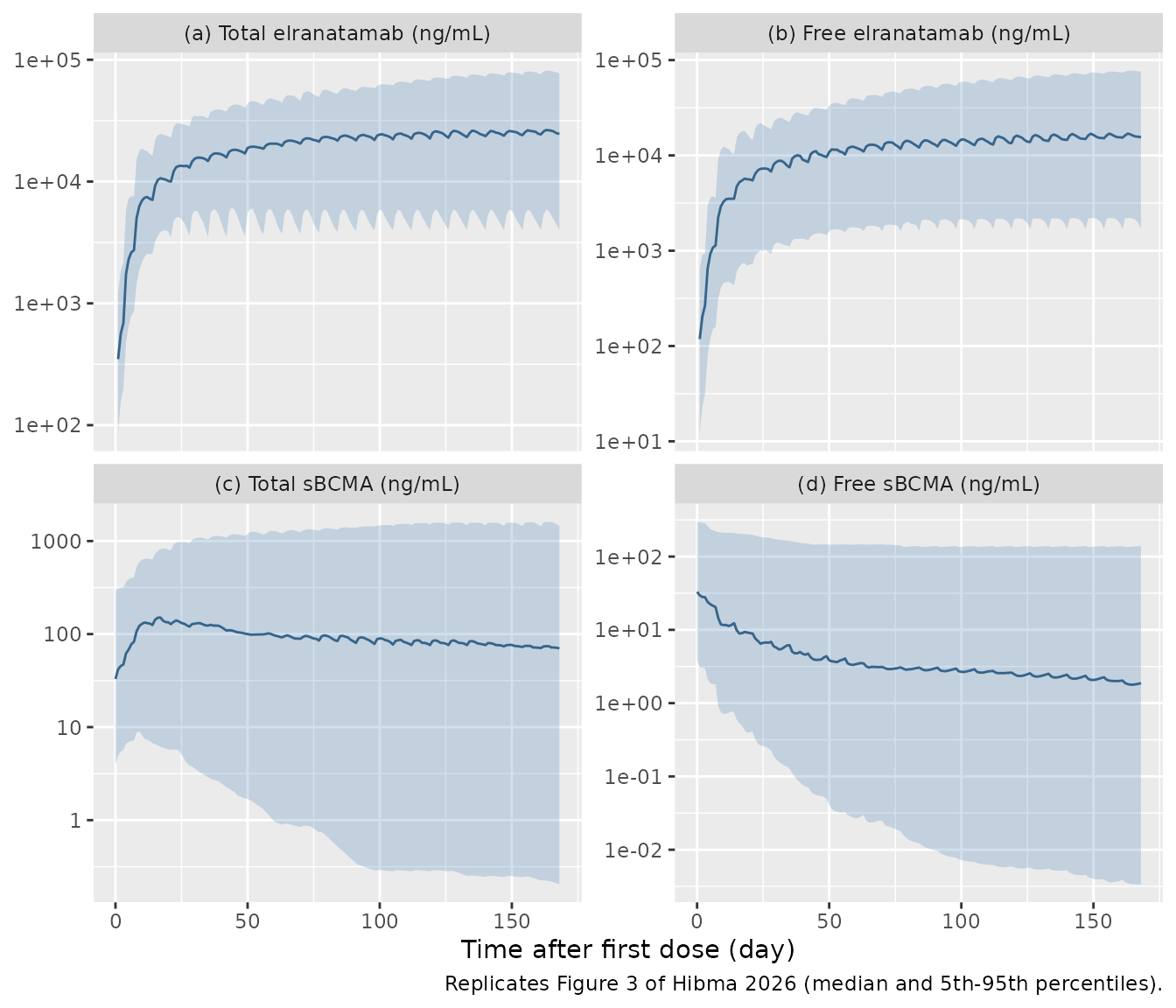
Figure 7 and Table 4: dose-interruption scenarios
Figure 7 shows the median free elranatamab profile when dosing stops after each of six scenarios. The threshold is 212 ng/mL, the geometric mean peak free concentration after the 12 mg first step-up dose. Table 4 lists the time from the last dose until the median falls below this threshold. It also lists the median concentration 84 days (12 weeks) after the last dose.
threshold <- 212
med <- sim |>
  group_by(scenario, last_dose, n76, time) |>
  summarise(Cc = median(Cc), .groups = "drop")

ggplot(med |> filter(Cc > 1), aes(time / 7, Cc, colour = scenario)) +
  geom_line() +
  geom_hline(yintercept = threshold, colour = "darkgreen") +
  scale_y_log10() +
  labs(x = "Time after first dose (weeks)", y = "Median free elranatamab (ng/mL)",
       colour = NULL,
       caption = "Replicates Figure 7 of Hibma 2026; green line = 212 ng/mL.") +
  theme(legend.position = "bottom", legend.direction = "vertical")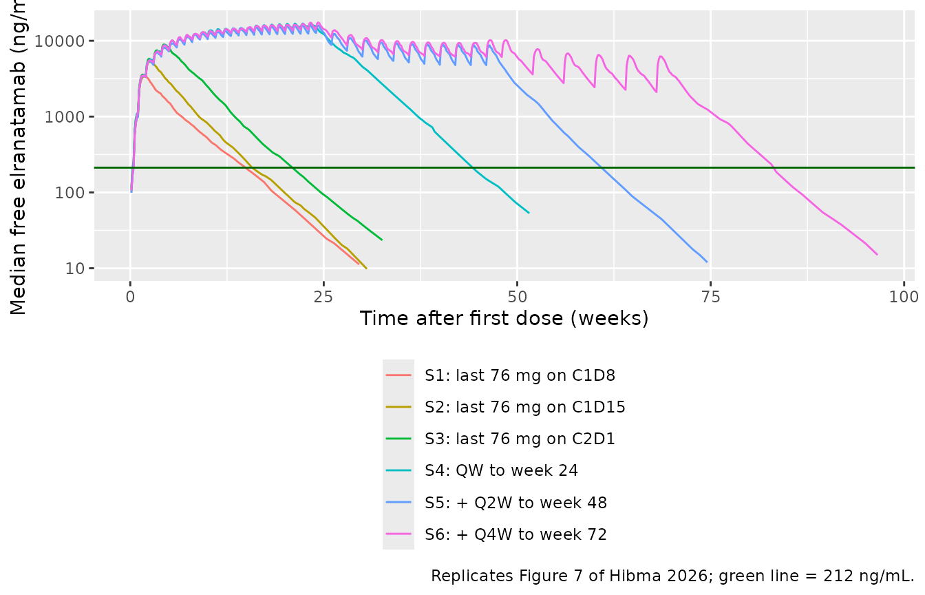
# Time after the last dose at which the median crosses the threshold, by
# log-linear interpolation between the bracketing daily grid points.
cross_time <- function(t, c, thr) {
  i <- which(c <= thr)[1]
  if (is.na(i) || i == 1L) return(NA_real_)
  t[i - 1] + (log(thr) - log(c[i - 1])) / (log(c[i]) - log(c[i - 1])) * (t[i] - t[i - 1])
}
tab4_pub <- tibble::tribble(
  ~scenario,                   ~n76_pub, ~t_pub, ~c84_pub,
  "S1: last 76 mg on C1D8",    1,        87.3,   231.9,
  "S2: last 76 mg on C1D15",   2,        103.5,  390.5,
  "S3: last 76 mg on C2D1",    4,        119.6,  697.1,
  "S4: QW to week 24",         23,       143.1,  1668.0,
  "S5: + Q2W to week 48",      35,       123.9,  863.0,
  "S6: + Q4W to week 72",      41,       107,    449.0
)
tab4 <- med |>
  filter(time > last_dose) |>
  group_by(scenario, n76, last_dose) |>
  summarise(
    t_sim = cross_time(time - last_dose, Cc, threshold),
    c84_sim = Cc[which.min(abs(time - last_dose - 84))],
    .groups = "drop"
  ) |>
  left_join(tab4_pub, by = "scenario") |>
  mutate(t_pct = 100 * (t_sim / t_pub - 1), c84_pct = 100 * (c84_sim / c84_pub - 1))

tab4 |>
  select(scenario, n76, t_pub, t_sim, t_pct, c84_pub, c84_sim, c84_pct) |>
  rename(
    "Scenario" = scenario, "76 mg doses" = n76,
    "Days to <= 212 ng/mL, paper" = t_pub, "Days, simulated" = t_sim, "Days % diff" = t_pct,
    "Conc. 84 d after last dose, paper (ng/mL)" = c84_pub,
    "Conc. 84 d, simulated" = c84_sim, "Conc. % diff" = c84_pct
  ) |>
knitr::kable(digits = 1, caption = "Reproduces Table 4 of Hibma 2026.")| Scenario | 76 mg doses | Days to <= 212 ng/mL, paper | Days, simulated | Days % diff | Conc. 84 d after last dose, paper (ng/mL) | Conc. 84 d, simulated | Conc. % diff |
|---|---|---|---|---|---|---|---|
| S1: last 76 mg on C1D8 | 1 | 87.3 | 97.3 | 11.4 | 231.9 | 297.2 | 28.2 |
| S2: last 76 mg on C1D15 | 2 | 103.5 | 96.4 | -6.9 | 390.5 | 329.1 | -15.7 |
| S3: last 76 mg on C2D1 | 4 | 119.6 | 118.6 | -0.8 | 697.1 | 570.2 | -18.2 |
| S4: QW to week 24 | 23 | 143.1 | 148.7 | 3.9 | 1668.0 | 1595.7 | -4.3 |
| S5: + Q2W to week 48 | 35 | 123.9 | 104.3 | -15.9 | 863.0 | 391.6 | -54.6 |
| S6: + Q4W to week 72 | 41 | 107.0 | 105.9 | -1.1 | 449.0 | 421.2 | -6.2 |
stopifnot(
  all(tab4$n76 == tab4$n76_pub),
  nrow(tab4) == 6L, !anyNA(tab4$t_sim),
  # The paper's conclusion: the median stays above the threshold for more
  # than 12 weeks in every scenario.
  all(tab4$t_sim > 84),
  # Structural envelope. The paper's medians come from post-hoc estimates of
  # the 321 analysed patients, ours from a fresh cohort. A mis-transcribed
  # CL, Vc, F or MW moves these times by tens of days.
  abs(median(tab4$t_pct)) < 15,
  max(abs(tab4$t_pct)) < 30
)
Days-to-threshold reproduces to within 16% in every scenario. The median difference is about 1%, and all six scenarios stay above 12 weeks, which is the paper’s conclusion. The 84-day concentrations agree less closely. They fall on the steep terminal decline, where shifting the curve by a few days moves the concentration by tens of percent.
PKNCA validation
Table 3: free elranatamab exposure metrics
Table 3 gives the geometric mean (GM) Caverage, Cmax and Ctrough of
free elranatamab over four dosing intervals of the full regimen: the
first full dose (Day 8), steady-state QW (week 24), Q2W (week 48) and
Q4W (week 72). Scenario S6 follows that regimen. PKNCA computes the
interval metrics. cmin stands in for Ctrough, because
PKNCA’s ctrough is undefined for an interval that does not
start at time 0. Results are pooled by GM to match the table.
s6 <- sim |> filter(scenario == "S6: + Q4W to week 72")
conc_df <- s6 |>
  filter(!is.na(Cc)) |>
  mutate(Cc = pmax(Cc, 0)) |>
  select(id, time, Cc, scenario)
conc_df <- bind_rows(
  conc_df,
  conc_df |> distinct(id, scenario) |> mutate(time = 0, Cc = 0)
) |>
  distinct(id, scenario, time, .keep_all = TRUE) |>
  arrange(id, scenario, time)
dose_df <- events |>
  filter(scenario == "S6: + Q4W to week 72", evid == 1) |>
  select(id, time, amt, scenario)

conc_obj <- PKNCA::PKNCAconc(conc_df, Cc ~ time | scenario + id)
dose_obj <- PKNCA::PKNCAdose(dose_df, amt ~ time | scenario + id)
intervals <- data.frame(
  start = c(7, 161, 322, 476),
  end = c(14, 168, 336, 504),
  cmax = TRUE, cav = TRUE, cmin = TRUE
)
nca_res <- PKNCA::pk.nca(PKNCA::PKNCAdata(conc_obj, dose_obj, intervals = intervals))
period_lab <- c(`7` = "First full dose (Day 8)", `161` = "SSQW (Week 24)",
                `322` = "SSQ2W (Week 48)", `476` = "SSQ4W (Week 72)")
gm <- function(x) exp(mean(log(x)))
sim_gm <- as.data.frame(nca_res$result) |>
  filter(PPTESTCD %in% c("cmax", "cav", "cmin")) |>
  mutate(period = unname(period_lab[as.character(start)])) |>
  group_by(period, PPTESTCD) |>
  summarise(PPORRES = gm(PPORRES), .groups = "drop")

published_t3 <- tibble::tribble(
  ~period,                    ~cav,     ~cmax,    ~cmin,
  "First full dose (Day 8)",  3083.46,  3794.53,  323.35,
  "SSQW (Week 24)",           32025.26, 33020.03, 30460.11,
  "SSQ2W (Week 48)",          17688.78, 19493.64, 15099.10,
  "SSQ4W (Week 72)",          8788.19,  11519.69, 5921.46
)
cmp <- nlmixr2lib::ncaComparisonTable(
  simulated = sim_gm, reference = published_t3, by = "period",
  units = c(cmax = "ng/mL", cav = "ng/mL", cmin = "ng/mL"),
  tolerance_pct = 20
)
knitr::kable(cmp, caption = "Geometric-mean free elranatamab exposure: simulated vs Hibma 2026 Table 3. * differs by >20%.")| NCA parameter | period | Reference | Simulated | % diff |
|---|---|---|---|---|
| Cmax (ng/mL) | First full dose (Day 8) | 3790 | 3490 | -8.1% |
| Cmax (ng/mL) | SSQW (Week 24) | 33000 | 16600 | -49.9%* |
| Cmax (ng/mL) | SSQ2W (Week 48) | 19500 | 10400 | -46.5%* |
| Cmax (ng/mL) | SSQ4W (Week 72) | 11500 | 6710 | -41.7%* |
| Cmin (ng/mL) | First full dose (Day 8) | 323 | 986 | +204.9%* |
| Cmin (ng/mL) | SSQW (Week 24) | 30500 | 14000 | -54.0%* |
| Cmin (ng/mL) | SSQ2W (Week 48) | 15100 | 6680 | -55.8%* |
| Cmin (ng/mL) | SSQ4W (Week 72) | 5920 | 2390 | -59.6%* |
| Cavg (ng/mL) | First full dose (Day 8) | 3080 | 2800 | -9.3% |
| Cavg (ng/mL) | SSQW (Week 24) | 32000 | 15600 | -51.2%* |
| Cavg (ng/mL) | SSQ2W (Week 48) | 17700 | 8880 | -49.8%* |
| Cavg (ng/mL) | SSQ4W (Week 72) | 8790 | 4600 | -47.7%* |
gm_ratio <- sim_gm |>
  left_join(pivot_longer(published_t3, -period, names_to = "PPTESTCD", values_to = "pub"),
            by = c("period", "PPTESTCD")) |>
  mutate(ratio = PPORRES / pub)
The first-full-dose Cmax and Caverage agree with Table 3 to within about 10%. Two groups of rows do not reproduce, and both are recorded as known deviations rather than tuned away:
- Steady-state rows (weeks 24, 48 and 72). The simulation gives about half the Table 3 geometric means. The paper is not self-consistent here. Its own Figure 7 median at week 24 is about 20,000 ng/mL, against a Table 3 GM of 32,025 ng/mL. Table 4, which this article reproduces closely (above), was simulated over all 321 patients. Table 3 summarises post-hoc estimates of the analysis population at those weeks. The patients still on treatment then are mostly responders with lower clearance, and the tight Table 3 CVs (46-60%, against a 100% CV on CL) point to that enriched subset. The paper itself excluded simulated subjects with CL > 0.3 L/day after about 84 days to reproduce this dropout in its pcVPCs (Section 2.7). The virtual cohort has no dropout.
-
First-full-dose Ctrough. Table 3 prints 323 ng/mL.
That is barely above the 212 ng/mL GM peak after the 12 mg dose,
although the 32 mg second step-up dose has been given in between. The
simulated Day 8 pre-dose value, which is PKNCA’s
cminover Days 8-15, is about three times higher. The paper does not define which trough this row holds, so the row is displayed and excluded from the gate.
gated <- gm_ratio |> filter(!(period == "First full dose (Day 8)" & PPTESTCD == "cmin"))
stopifnot(
  nrow(gm_ratio) == 12L, !anyNA(gm_ratio$ratio), nrow(gated) == 11L,
  # First full dose: every patient contributes, so no enrichment.
  all(abs(gated$ratio[gated$period == "First full dose (Day 8)"] - 1) < 0.35),
  # Later intervals: the simulation must not EXCEED the enriched table and
  # must stay within a factor of 3 of it (realised 0.40-0.58).
  all(gated$ratio > 1 / 3), all(gated$ratio < 1.3)
)
Accumulation, dose proportionality and baseline sBCMA (Figure 5)
The paper gives median accumulation ratios for 76 mg QW. For Cmax they are 4.8 (total) and 6.6 (free); for AUCtau they are 8.0 (total) and 11.2 (free). Figure 5 regresses log free AUCtau on log dose over 6-76 mg SC QW. The slopes are about 1.0-1.2 overall. At steady state the slope rises to about 1.6 for patients above the 90th percentile of baseline sBCMA, where the shed-target sink saturates.
The accumulation ratios are medians over 200 virtual patients receiving 76 mg QW from the first dose. Each ratio is steady state (week 24) over the first dose. The typical male is shown alongside. Females (half the clearance) accumulate more than the typical male, so the cohort median sits above him. The dose-proportionality slopes use typical values at the 10th and 90th percentiles of the model’s baseline sBCMA distribution. At the 90th percentile that is 6.914 * exp(1.2816 * 1.3461) = 38.9 nM, and these slopes are deterministic. A small stochastic cohort then gives the population picture.
auc_tau <- function(s, from, to, col) {
  d <- s[s$time >= from & s$time <= to, ]
  sum(diff(d$time) * (head(d[[col]], -1) + tail(d[[col]], -1)) / 2)
}
acc_ratios <- function(s) {
  c(
    cmax_total = max(s$Cc_total[s$time >= 161]) / max(s$Cc_total[s$time <= 7]),
    cmax_free = max(s$Cc[s$time >= 161]) / max(s$Cc[s$time <= 7]),
    auc_total = auc_tau(s, 161, 168, "Cc_total") / auc_tau(s, 0, 7, "Cc_total"),
    auc_free = auc_tau(s, 161, 168, "Cc") / auc_tau(s, 0, 7, "Cc")
  )
}
grid <- sort(unique(c(seq(0, 7, 0.05), seq(7, 161, 1), seq(161, 168, 0.05))))
s76 <- make_events(1L, seq(0, 161, 7), rep(76, 24), grid) |> typical_covs() |> solve_typ()
#> ℹ omega/sigma items treated as zero: 'etalcl', 'etalvc', 'etalvp', 'etalq', 'etalka', 'etalfdepot', 'etalcl_target', 'etalvc_target', 'etalrbase_target', 'etalcl_complex', 'etalvc_complex', 'etalkd'

rxode2::rxSetSeed(76)
ev_acc <- make_events(seq_len(200), seq(0, 161, 7), rep(76, 24), grid) |>
  left_join(draw_covs(200) |> mutate(id = seq_len(200)), by = "id")
sim_acc <- rxode2::rxSolve(mod_pk, events = ev_acc, returnType = "data.frame",
                           useLinCmt = FALSE) |>
  as.data.frame()
acc_cohort <- sim_acc |>
  group_by(id) |>
  group_modify(~ as.data.frame(t(acc_ratios(.x)))) |>
  ungroup()

acc <- tibble::tibble(
  metric = c("Cmax, total", "Cmax, free", "AUCtau, total", "AUCtau, free"),
  typical = acc_ratios(s76),
  cohort = vapply(acc_cohort[, -1], median, numeric(1)),
  paper = c(4.8, 6.6, 8.0, 11.2)
)
acc |>
  rename("Accumulation ratio (76 mg QW, week 24 / first dose)" = metric,
         "Typical male" = typical, "Cohort median" = cohort,
         "Hibma 2026 (median)" = paper) |>
knitr::kable(digits = 2)| Accumulation ratio (76 mg QW, week 24 / first dose) | Typical male | Cohort median | Hibma 2026 (median) |
|---|---|---|---|
| Cmax, total | 3.42 | 4.75 | 4.8 |
| Cmax, free | 5.40 | 6.41 | 6.6 |
| AUCtau, total | 4.28 | 5.87 | 8.0 |
| AUCtau, free | 7.26 | 8.09 | 11.2 |
# The per-patient ratios are heavily right-skewed (interquartile range about
# 3-10 for AUCtau, total), so a 200-patient median is noisy: two cohorts
# drawn while writing this article gave cohort/paper ratios of 0.72-0.99 and
# 0.94-1.43 across the four rows. The bound admits that spread; the typical
# male, a deterministic floor, sits 35-46% below the paper for AUCtau.
stopifnot(all(abs(log(acc$cohort / acc$paper)) < log(1.6)))
Here the four cohort medians fall within 30% of the paper’s medians. Another 200-patient cohort drawn while writing this article landed up to 43% above them, so the spread between one cohort and the next is as large as the difference from the paper. It comes from the long right tail created by the 100% CV on elranatamab clearance and the 448% CV on sBCMA clearance. The paper’s medians were taken over the post-hoc estimates of 321 patients, so they carry the same kind of sampling noise.
dp_doses <- c(6, 10, 16, 28, 44, 60, 76)
slope_at <- function(model) {
  res <- vapply(dp_doses, function(d) {
    s <- make_events(1L, seq(0, 161, 7), rep(d, 24), grid) |> typical_covs() |>
      solve_typ(model = model)
    c(sd = auc_tau(s, 0, 7, "Cc"), ss = auc_tau(s, 161, 168, "Cc"))
  }, numeric(2))
  c(single = unname(coef(lm(log(res["sd", ]) ~ log(dp_doses)))[2]),
    ss = unname(coef(lm(log(res["ss", ]) ~ log(dp_doses)))[2]))
}
bl90 <- exp(th[["lrbase_target"]] + qnorm(0.9) * sqrt(om[["etalrbase_target"]]))
bl10 <- exp(th[["lrbase_target"]] + qnorm(0.1) * sqrt(om[["etalrbase_target"]]))
slopes <- rbind(
  "BL sBCMA 10th percentile" = slope_at(mod_typ |> rxode2::ini(lrbase_target = log(bl10))),
  "BL sBCMA typical (6.914 nM)" = slope_at(mod_typ),
  "BL sBCMA 90th percentile" = slope_at(mod_typ |> rxode2::ini(lrbase_target = log(bl90)))
)
#> ℹ change initial estimate of `lrbase_target` to `0.208449498966833`
#> ℹ omega/sigma items treated as zero: 'etalcl', 'etalvc', 'etalvp', 'etalq', 'etalka', 'etalfdepot', 'etalcl_target', 'etalvc_target', 'etalrbase_target', 'etalcl_complex', 'etalvc_complex', 'etalkd'
#> ℹ omega/sigma items treated as zero: 'etalcl', 'etalvc', 'etalvp', 'etalq', 'etalka', 'etalfdepot', 'etalcl_target', 'etalvc_target', 'etalrbase_target', 'etalcl_complex', 'etalvc_complex', 'etalkd'
#> ℹ omega/sigma items treated as zero: 'etalcl', 'etalvc', 'etalvp', 'etalq', 'etalka', 'etalfdepot', 'etalcl_target', 'etalvc_target', 'etalrbase_target', 'etalcl_complex', 'etalvc_complex', 'etalkd'
#> ℹ omega/sigma items treated as zero: 'etalcl', 'etalvc', 'etalvp', 'etalq', 'etalka', 'etalfdepot', 'etalcl_target', 'etalvc_target', 'etalrbase_target', 'etalcl_complex', 'etalvc_complex', 'etalkd'
#> ℹ omega/sigma items treated as zero: 'etalcl', 'etalvc', 'etalvp', 'etalq', 'etalka', 'etalfdepot', 'etalcl_target', 'etalvc_target', 'etalrbase_target', 'etalcl_complex', 'etalvc_complex', 'etalkd'
#> ℹ omega/sigma items treated as zero: 'etalcl', 'etalvc', 'etalvp', 'etalq', 'etalka', 'etalfdepot', 'etalcl_target', 'etalvc_target', 'etalrbase_target', 'etalcl_complex', 'etalvc_complex', 'etalkd'
#> ℹ omega/sigma items treated as zero: 'etalcl', 'etalvc', 'etalvp', 'etalq', 'etalka', 'etalfdepot', 'etalcl_target', 'etalvc_target', 'etalrbase_target', 'etalcl_complex', 'etalvc_complex', 'etalkd'
#> ℹ omega/sigma items treated as zero: 'etalcl', 'etalvc', 'etalvp', 'etalq', 'etalka', 'etalfdepot', 'etalcl_target', 'etalvc_target', 'etalrbase_target', 'etalcl_complex', 'etalvc_complex', 'etalkd'
#> ℹ omega/sigma items treated as zero: 'etalcl', 'etalvc', 'etalvp', 'etalq', 'etalka', 'etalfdepot', 'etalcl_target', 'etalvc_target', 'etalrbase_target', 'etalcl_complex', 'etalvc_complex', 'etalkd'
#> ℹ omega/sigma items treated as zero: 'etalcl', 'etalvc', 'etalvp', 'etalq', 'etalka', 'etalfdepot', 'etalcl_target', 'etalvc_target', 'etalrbase_target', 'etalcl_complex', 'etalvc_complex', 'etalkd'
#> ℹ omega/sigma items treated as zero: 'etalcl', 'etalvc', 'etalvp', 'etalq', 'etalka', 'etalfdepot', 'etalcl_target', 'etalvc_target', 'etalrbase_target', 'etalcl_complex', 'etalvc_complex', 'etalkd'
#> ℹ omega/sigma items treated as zero: 'etalcl', 'etalvc', 'etalvp', 'etalq', 'etalka', 'etalfdepot', 'etalcl_target', 'etalvc_target', 'etalrbase_target', 'etalcl_complex', 'etalvc_complex', 'etalkd'
#> ℹ omega/sigma items treated as zero: 'etalcl', 'etalvc', 'etalvp', 'etalq', 'etalka', 'etalfdepot', 'etalcl_target', 'etalvc_target', 'etalrbase_target', 'etalcl_complex', 'etalvc_complex', 'etalkd'
#> ℹ omega/sigma items treated as zero: 'etalcl', 'etalvc', 'etalvp', 'etalq', 'etalka', 'etalfdepot', 'etalcl_target', 'etalvc_target', 'etalrbase_target', 'etalcl_complex', 'etalvc_complex', 'etalkd'
#> ℹ change initial estimate of `lrbase_target` to `3.65864718403203`
#> ℹ omega/sigma items treated as zero: 'etalcl', 'etalvc', 'etalvp', 'etalq', 'etalka', 'etalfdepot', 'etalcl_target', 'etalvc_target', 'etalrbase_target', 'etalcl_complex', 'etalvc_complex', 'etalkd'
#> ℹ omega/sigma items treated as zero: 'etalcl', 'etalvc', 'etalvp', 'etalq', 'etalka', 'etalfdepot', 'etalcl_target', 'etalvc_target', 'etalrbase_target', 'etalcl_complex', 'etalvc_complex', 'etalkd'
#> ℹ omega/sigma items treated as zero: 'etalcl', 'etalvc', 'etalvp', 'etalq', 'etalka', 'etalfdepot', 'etalcl_target', 'etalvc_target', 'etalrbase_target', 'etalcl_complex', 'etalvc_complex', 'etalkd'
#> ℹ omega/sigma items treated as zero: 'etalcl', 'etalvc', 'etalvp', 'etalq', 'etalka', 'etalfdepot', 'etalcl_target', 'etalvc_target', 'etalrbase_target', 'etalcl_complex', 'etalvc_complex', 'etalkd'
#> ℹ omega/sigma items treated as zero: 'etalcl', 'etalvc', 'etalvp', 'etalq', 'etalka', 'etalfdepot', 'etalcl_target', 'etalvc_target', 'etalrbase_target', 'etalcl_complex', 'etalvc_complex', 'etalkd'
#> ℹ omega/sigma items treated as zero: 'etalcl', 'etalvc', 'etalvp', 'etalq', 'etalka', 'etalfdepot', 'etalcl_target', 'etalvc_target', 'etalrbase_target', 'etalcl_complex', 'etalvc_complex', 'etalkd'
#> ℹ omega/sigma items treated as zero: 'etalcl', 'etalvc', 'etalvp', 'etalq', 'etalka', 'etalfdepot', 'etalcl_target', 'etalvc_target', 'etalrbase_target', 'etalcl_complex', 'etalvc_complex', 'etalkd'
knitr::kable(slopes, digits = 2,
caption = "Typical-value slope of log(free AUCtau) on log(dose), 6-76 mg SC QW (Figure 5 reports about 1.0-1.2, and 1.6 at steady state for the upper sBCMA decile).")| single | ss | |
|---|---|---|
| BL sBCMA 10th percentile | 1.05 | 1.02 |
| BL sBCMA typical (6.914 nM) | 1.17 | 1.14 |
| BL sBCMA 90th percentile | 1.10 | 1.63 |
# Stochastic cohort, 60 per dose level, for the Figure 5 display.
trap <- function(t, c) sum(diff(t) * (head(c, -1) + tail(c, -1)) / 2)
grid_dp <- sort(unique(c(seq(0, 7, 0.25), seq(161, 168, 0.25))))
ev_dp <- bind_rows(lapply(seq_along(dp_doses), function(i) {
  ids <- (i - 1L) * 60L + seq_len(60)
  make_events(ids, seq(0, 161, 7), rep(dp_doses[i], 24), grid_dp) |>
    left_join(draw_covs(60) |> mutate(id = ids), by = "id") |>
    mutate(dose = dp_doses[i])
}))
sim_dp <- rxode2::rxSolve(mod_pk, events = ev_dp, keep = "dose",
                          returnType = "data.frame", useLinCmt = FALSE) |>
  as.data.frame()
# AUC in nM*day, as in Figure 5 (ng/mL / 148 = nM).
auc_dp <- sim_dp |>
  group_by(id, dose) |>
  summarise(
    rbase = first(rbase_target),
    `Single dose` = trap(time[time <= 7], Cc[time <= 7]) / 148,
    `Steady state` = trap(time[time >= 161], Cc[time >= 161]) / 148,
    .groups = "drop"
  )
bl_cut <- quantile(auc_dp$rbase, c(0.1, 0.9))
auc_dp <- auc_dp |>
  mutate(bl_group = case_when(
    rbase <= bl_cut[1] ~ "BL sBCMA <= 10th pct",
    rbase >= bl_cut[2] ~ "BL sBCMA >= 90th pct",
    TRUE ~ "BL sBCMA 10th-90th pct"
  ), bl_group = factor(bl_group, c("BL sBCMA <= 10th pct", "BL sBCMA 10th-90th pct", "BL sBCMA >= 90th pct"))) |>
  pivot_longer(c(`Single dose`, `Steady state`), names_to = "period", values_to = "auc")

ggplot(auc_dp, aes(dose, auc)) +
  geom_point(alpha = 0.3, size = 0.8) +
  geom_smooth(method = "lm", formula = y ~ x, se = FALSE, colour = "black") +
  facet_grid(period ~ bl_group, scales = "free_y") +
  scale_x_log10(breaks = dp_doses) +
  scale_y_log10() +
  labs(x = "Dose (mg)", y = "Free elranatamab AUCtau (nM*day)",
       caption = "Replicates Figure 5 of Hibma 2026 (simulated cohort, 60 per dose).")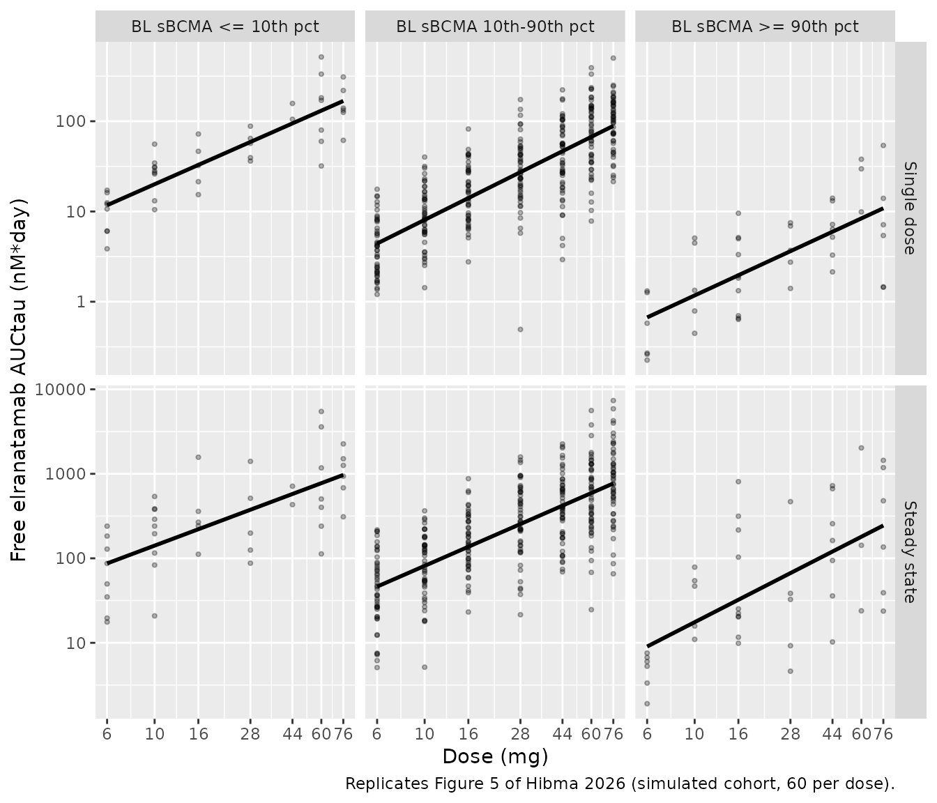
auc_dp |>
  group_by(period, bl_group) |>
  summarise(slope = unname(coef(lm(log(auc) ~ log(dose)))[2]), .groups = "drop") |>
  pivot_wider(names_from = period, values_from = slope) |>
  rename("Baseline sBCMA group" = bl_group) |>
knitr::kable(digits = 2, caption = "Cohort slopes of log(free AUCtau) on log(dose). Figure 5 reports single-dose 1.0 / 1.2 / 1.1 and steady-state 1.0 / 1.1 / 1.6 by group.")| Baseline sBCMA group | Single dose | Steady state |
|---|---|---|
| BL sBCMA <= 10th pct | 1.05 | 0.95 |
| BL sBCMA 10th-90th pct | 1.18 | 1.11 |
| BL sBCMA >= 90th pct | 1.10 | 1.30 |
The cohort slopes are shown for display only. About 42 patients fall in each tail group, so a slope carries a standard error of roughly 0.2. The gate on the sBCMA effect is the typical-value calculation above.
Exposure by sex (Figure 2a)
Sex is the largest covariate effect: female clearance is 50.8% of male clearance. The paper reports median free AUCtau,ss of 1.33 in females and 0.579 in males, printed in “mg/L”. That unit cannot be an AUC. At 76 mg QW the steady-state free Caverage alone is about 16 mg/L for a typical male, so the absolute values could not be reconciled. The ratio, 2.30, is compared instead.
auc_sex <- sim |>
  filter(scenario == "S4: QW to week 24", time >= 161, time <= 168) |>
  group_by(id, SEXF) |>
  summarise(auc = trap(time, Cc), .groups = "drop") |>
  group_by(SEXF) |>
  summarise(median_auc = median(auc) / 1000, n = n(), .groups = "drop") |>
  mutate(sex = ifelse(SEXF == 1, "Female", "Male"))
typ_f <- make_events(1L, c(0, 3, qw), c(12, 32, rep(76, length(qw))), seq(161, 168, 0.25)) |>
  typical_covs(SEXF = 1) |> solve_typ()
#> ℹ omega/sigma items treated as zero: 'etalcl', 'etalvc', 'etalvp', 'etalq', 'etalka', 'etalfdepot', 'etalcl_target', 'etalvc_target', 'etalrbase_target', 'etalcl_complex', 'etalvc_complex', 'etalkd'
typ_m <- make_events(1L, c(0, 3, qw), c(12, 32, rep(76, length(qw))), seq(161, 168, 0.25)) |>
  typical_covs(SEXF = 0) |> solve_typ()
#> ℹ omega/sigma items treated as zero: 'etalcl', 'etalvc', 'etalvp', 'etalq', 'etalka', 'etalfdepot', 'etalcl_target', 'etalvc_target', 'etalrbase_target', 'etalcl_complex', 'etalvc_complex', 'etalkd'
typ_ratio <- trap(typ_f$time, typ_f$Cc) / trap(typ_m$time, typ_m$Cc)
auc_sex |>
  select(sex, n, median_auc) |>
  rename("Sex" = sex, "N simulated" = n, "Median free AUCtau,ss week 24 (mg*day/L)" = median_auc) |>
knitr::kable(digits = 1)| Sex | N simulated | Median free AUCtau,ss week 24 (mg*day/L) |
|---|---|---|
| Male | 77 | 89.4 |
| Female | 73 | 144.9 |
The typical-value female-to-male ratio of free AUCtau at week 24 is 1.89. The simulated-cohort ratio of medians is 1.62. The paper’s ratio of medians is 2.30.
# Deterministic: at steady state free exposure scales ~1/CL, and female CL is
# (1 - 0.492) of male, so the typical ratio sits just under 1/0.508 = 1.97.
stopifnot(typ_ratio > 1.7, typ_ratio < 2.1)
CRS exposure-response (Figure 6)
The CRS model needs the free elranatamab concentration on Day 4, just before the 32 mg second step-up dose. That value is also the peak of the first step-up interval. The simulated cohorts all start with the same 12 mg dose, so all 900 virtual patients contribute. Their geometric mean is compared with the 212 ng/mL (90% CV) the paper reports as the geometric mean peak after the first step-up dose. The CRS probability is then evaluated with baseline tumour burden drawn at the MagnetisMM-3 rate (38 high of 169 with a known value).
day4 <- sim |>
  filter(time == 3) |>
  distinct(id, .keep_all = TRUE) |>
  transmute(id, CTROUGH = Cc)
gm_day4 <- exp(mean(log(day4$CTROUGH)))
gcv_day4 <- 100 * sqrt(exp(var(log(day4$CTROUGH))) - 1)
c(geometric_mean = gm_day4, geometric_cv_pct = gcv_day4)
#>   geometric_mean geometric_cv_pct
#>         198.6606         150.4409

# Structural: F, ka, Vc and the MW conversion all enter the Day 4 value; an
# error in any of them moves the GM by far more than 35%.
stopifnot(nrow(day4) == 6L * n_per, abs(gm_day4 / 212 - 1) < 0.35)
The geometric mean is close to 212 ng/mL. The simulated geometric CV is wider than the paper’s 90%. That is expected: the virtual cohort samples the full population IIV, whereas the paper’s figure comes from post-hoc estimates, which shrinkage (up to 31% here) pulls towards the typical value.
rxode2::rxSetSeed(6)
crs_ev <- day4 |>
  mutate(time = 0, amt = 0, evid = 0L,
         TUM_BURDEN_HIGH = rbinom(n(), 1, 38 / 169))
crs <- rxode2::rxSolve(mod_crs, events = crs_ev, keep = c("CTROUGH", "TUM_BURDEN_HIGH"),
                       returnType = "data.frame") |>
  as.data.frame()
#> Warning: multi-subject simulation without without 'omega'
mean_p <- mean(crs$prob_crs_stepup1)
c(mean_predicted_probability = mean_p, observed_incidence = 79 / 183)
#> mean_predicted_probability         observed_incidence
#>                  0.4706519                  0.4316940
# A logistic regression's mean fitted probability equals the observed rate in
# its own data (79/183 = 43%). A fresh cohort drawn from the PK model is not
# the fitted data, so allow 12 percentage points; a unit error in CTROUGH
# (nM instead of ng/mL) would move this by more than 40 points.
stopifnot(abs(mean_p - 79 / 183) < 0.12)
grid_log <- seq(3.5, 7.1, length.out = 100)
curve_ev <- data.frame(id = 1L, time = seq_along(grid_log), amt = 0, evid = 0L,
                       CTROUGH = exp(grid_log), TUM_BURDEN_HIGH = 0)
curve <- rxode2::rxSolve(mod_crs, events = curve_ev, returnType = "data.frame") |>
  as.data.frame() |>
  mutate(log_ctrough = grid_log)
p6a <- ggplot(curve, aes(log_ctrough, prob_crs_stepup1)) +
  geom_line(colour = "blue") +
  geom_rug(data = crs, aes(x = log(CTROUGH)), inherit.aes = FALSE, alpha = 0.2) +
  coord_cartesian(ylim = c(0, 1)) +
  labs(x = "Log(Ctrough [ng/mL])", y = "Predicted probability",
       title = "(a) Any-grade CRS after the first step-up dose, low/intermediate tumour burden",
       caption = "Replicates Figure 6a of Hibma 2026; rug = simulated Day 4 exposures.")
p6a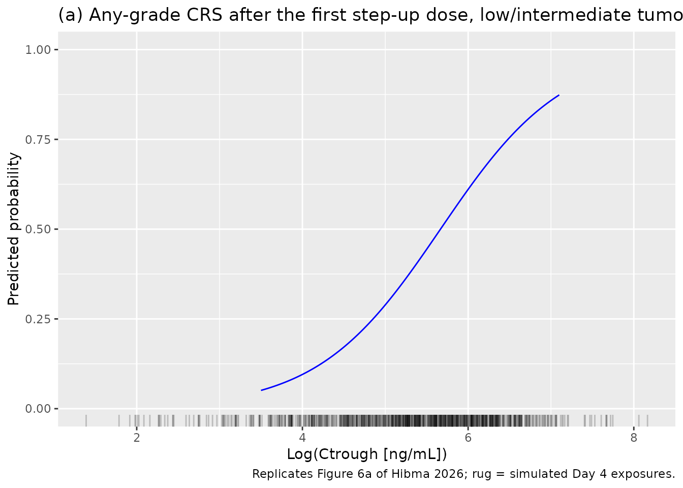
# Figure 6b: exposure in patients with and without CRS, drawing each virtual
# patient's outcome from its predicted probability.
crs$CRS <- ifelse(rbinom(nrow(crs), 1, crs$prob_crs_stepup1) == 1, "Yes", "No")
ggplot(crs, aes(CRS, log(CTROUGH))) +
  geom_boxplot(outlier.shape = NA) +
  geom_jitter(width = 0.15, alpha = 0.2, colour = "seagreen") +
  labs(x = "Any-grade CRS after the first step-up dose", y = "Log(Ctrough [ng/mL])",
       caption = "Replicates Figure 6b of Hibma 2026 (simulated outcomes).")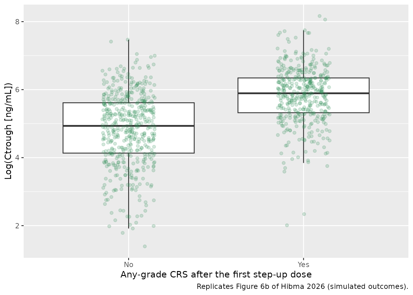
Assumptions and deviations
-
sBCMA synthesis rate and initial condition. The
paper writes
ksynin the dA4/dt equation but does not give its value. It estimates the baseline sBCMA concentration BLsBCMA instead. The model setsksyn = CLsBCMA * BLsBCMAandtotal_target(0) = BLsBCMA * Vc,sBCMA, which is the drug-free steady state. This is the only reading under which BLsBCMA is the baseline, and the steady-state chunk above confirms that sBCMA stays at 6.914 nM without drug. -
IIV scale. Table 2’s “CV (%)” is
100 * sqrt(omega^2), which the confidence-interval check above demonstrates. Variances are(CV/100)^2, including a variance of 20.08 for sBCMA clearance. IIV is exponential on every parameter, bioavailability included, as stated in Methods. The paper does not say whether F was logit-transformed. With a 14.8% CV individual F exceeds 1 only beyond about 4 SD. - IIV held at a small value. The Methods quote a variance of 0.025 for the IIVs held at a small value (Vp, Q, F, Kd). Table 2 prints them as 14.83% CV, which is a variance of 0.022, and the model uses the table value.
- Residual error. Table 2 lists the four proportional residual terms among the fixed effects with RSEs. They are taken to be SD-scale thetas (SAEM Mu-referencing with SIGMA fixed to 1) and encoded as proportional SDs.
-
Complex amount. Section 2.4 prints the complex
amount as the smaller root
0.5 * (b - sqrt(b^2 - 4 * A1 * A4)). The model uses the identical rationalised form2 * A1 * A4 / (b + sqrt(b^2 - 4 * A1 * A4)). The printed form subtracts two nearly equal numbers once the drug has washed out, and loses precision there; the rationalised form does not. -
Units. The model works in molar units internally,
as the paper does (148 kDa for elranatamab). Doses are given in mg to
depot(SC) orcentral(IV). The drug states are carried in mg and converted to nmol insidemodel(). Free and total elranatamab are reported in ng/mL; free and total sBCMA are reported in nM, which is how the model was fitted and how Table 1 reports baseline sBCMA (x 5.4 for ng/mL). - Table 2 typo. The printed 95% CI for “Age on ka” is “(2.031; -0.886)”. The lower bound has lost its minus sign. The estimate -1.459 is used.
- Reference weight. The Vc equation centres body weight at 71.45 kg, and that value is used. Table 1 reports the median as 71.50 kg.
- Missing tumour burden. ESM Table S2 prints a single “TumorBurden High” coefficient against a low/intermediate reference. The paper does not say how the 14 patients with missing tumour burden were coded. The virtual cohort draws high burden at 38/169 among patients with a known value.
- Virtual cohort. The dose-interruption simulations in the paper used post-hoc estimates of the 321 analysed patients. This article uses fresh draws from the population distribution, with covariates approximating Table 1 (48% female; weight log-normal around 71.5 kg; age around 65 years). There is no dropout, so late-interval exposures sit below the enriched post-hoc summaries of Table 3 (discussed above).
-
Placeholder residual on the CRS model. The CRS
model is a Bernoulli logistic regression with no residual error.
addSd_prob_crs_stepup1 = 0.001is a fixed placeholder so that rxode2 has an error model. It is not a published value. - No correction notice was found for Hibma 2026 as of 2026-09-29.