Shikimic acid PK and antioxidant PD in broilers (Shen 2026)
Source:vignettes/articles/Shen_2026_shikimicAcid.Rmd
Shen_2026_shikimicAcid.RmdModel and source
Shikimic acid (SA) is a highly polar polyhydroxy cyclic organic acid, best known as the synthetic precursor of oseltamivir but of independent interest as an “indirect” antioxidant that acts by activating the Nrf2/Keap1 pathway rather than by scavenging radicals directly. Shen 2026 is the first report of its pharmacokinetics in poultry.
Sixteen healthy 5-week-old yellow-feathered broilers were randomised to a single 50 mg/kg dose of SA given either intravenously (wing vein) or by oral gavage, n = 8 per group. Plasma SA was measured by HPLC-MS/MS. In the oral group only, serum total antioxidant capacity (T-AOC), superoxide dismutase (SOD) activity and malondialdehyde (MDA) were measured at 0, 1, 2, 4, 6, 8 and 12 h.
T-AOC and SOD rose and MDA fell, but all three peaked well after the
plasma peak, producing hysteresis loops (counter-clockwise for T-AOC and
SOD, clockwise for MDA). The authors therefore linked plasma to an
effect compartment and drove an
indirect-response turnover model from the effect-site
concentration, fitting each bird individually in Phoenix WinNonlin. Each
biomarker was fitted separately, with its own ke0,
S, kin and kout (Table 5), so the
paper contributes three model files that share one
plasma description:
sa_models <- c(
  "Shen_2026_shikimicAcid_broiler_taoc",  # T-AOC: SA stimulates production (kin)
  "Shen_2026_shikimicAcid_broiler_sod",   # SOD:   SA stimulates production (kin)
  "Shen_2026_shikimicAcid_broiler_mda"    # MDA:   SA stimulates loss       (kout)
)
# Parse each model once; the parsed object exposes the file-level metadata
# (reference, description, population) as well as being solvable.
mods <- lapply(sa_models, function(x) rxode2::rxode(readModelDb(x)))
names(mods) <- sa_models
vapply(mods, function(m) paste(m$state, collapse = ", "), character(1))
#> Shen_2026_shikimicAcid_broiler_taoc  Shen_2026_shikimicAcid_broiler_sod
#>      "depot, central, effect, taoc"       "depot, central, effect, sod"
#>  Shen_2026_shikimicAcid_broiler_mda
#> "depot, central, effect, mda"- Citation: Shen Y, Mo K, Zhao H, Zhang Y, Huang X (2026). Pharmacokinetic-pharmacodynamic integration of shikimic acid in broilers: An indirect effect modeling approach. Poultry Science 105:106959. doi:10.1016/j.psj.2026.106959
- Article: Poultry Science 2026;105:106959
Population
pop <- mods[[1]]$population
data.frame(
  Field = c("Species", "Subjects (oral arm)", "Age", "Body weight", "Sex",
            "Health status", "Dose", "Region"),
  Value = c(pop$species, as.character(pop$n_subjects), pop$age_median,
            pop$weight_range, pop$sex, pop$disease_state, pop$dose_range,
            pop$regions)
) |>
knitr::kable()| Field | Value |
|---|---|
| Species | chicken (yellow-feathered broiler) |
| Subjects (oral arm) | 8 |
| Age | 5 weeks |
| Body weight | mean initial body weight 1.98 +/- 0.11 kg (all 16 birds) |
| Sex | equal numbers of males and females |
| Health status | healthy broilers; no oxidative-stress challenge was applied |
| Dose | shikimic acid 50 mg/kg as a single oral (gavage) dose |
| Region | China |
Every parameter is fixed at the published mean of the eight individual fits. Shen 2026 reports only means and SDs of individual estimates, never an omega matrix, so there is no between-subject variability to simulate and the model is deterministic. A single typical-value profile is therefore the complete prediction; no virtual cohort is drawn.
Source trace
tribble(
  ~Quantity, ~`Source location`, ~Value,
  "Dose, route, species, n",        "Methods, 'Animals' / 'Dosing and sample collection'", "50 mg/kg PO gavage, broiler, n = 8",
  "dCe/dt = ke0 * (Cp - Ce)",       "Methods, 'Statistical analysis and PK-PD modeling'",  "effect-compartment link",
  "dE/dt = kin*(1+S*Ce) - kout*E",  "Methods, same section (T-AOC, SOD)",                  "stimulation of production",
  "dE/dt = kin - kout*(1+S*Ce)*E",  "Methods, same section (MDA)",                         "stimulation of loss",
  "E0 = kin/kout",                  "Methods, same section",                               "stated explicitly",
  "T-AOC ke0, S, kin, kout",        "Table 5, T-AOC row",                                  "0.44, 0.01, 0.37, 0.14",
  "SOD ke0, S, kin, kout",          "Table 5, SOD row",                                    "0.89, 0.04, 8.98, 0.31",
  "MDA ke0, S, kin, kout",          "Table 5, MDA row",                                    "1.06, 0.01, 0.84, 0.24",
  "CL/F = Dose/AUC_po",             "Table 4 (AUC 132.04 h*ug/mL)",                        "378.67 mL/h/kg",
  "V/F = Vz/F",                     "Table 3 (Vz 0.35 L/kg), Table 4 (F 40.37%)",          "866.98 mL/kg",
  "ka",                             "RECONSTRUCTED - not published (see Errata)",          "1.2378 /h",
  "Residual error structures",      "Methods, 'Statistical analysis and PK-PD modeling'",  "multiplicative PK, additive PD",
  "Residual error magnitudes",      "NOT reported (only initial SDs 0.1 / 1.0)",           "fixed at 0"
) |>
knitr::kable()| Quantity | Source location | Value |
|---|---|---|
| Dose, route, species, n | Methods, ‘Animals’ / ‘Dosing and sample collection’ | 50 mg/kg PO gavage, broiler, n = 8 |
| dCe/dt = ke0 * (Cp - Ce) | Methods, ‘Statistical analysis and PK-PD modeling’ | effect-compartment link |
| dE/dt = kin(1+SCe) - kout*E | Methods, same section (T-AOC, SOD) | stimulation of production |
| dE/dt = kin - kout(1+SCe)*E | Methods, same section (MDA) | stimulation of loss |
| E0 = kin/kout | Methods, same section | stated explicitly |
| T-AOC ke0, S, kin, kout | Table 5, T-AOC row | 0.44, 0.01, 0.37, 0.14 |
| SOD ke0, S, kin, kout | Table 5, SOD row | 0.89, 0.04, 8.98, 0.31 |
| MDA ke0, S, kin, kout | Table 5, MDA row | 1.06, 0.01, 0.84, 0.24 |
| CL/F = Dose/AUC_po | Table 4 (AUC 132.04 h*ug/mL) | 378.67 mL/h/kg |
| V/F = Vz/F | Table 3 (Vz 0.35 L/kg), Table 4 (F 40.37%) | 866.98 mL/kg |
| ka | RECONSTRUCTED - not published (see Errata) | 1.2378 /h |
| Residual error structures | Methods, ‘Statistical analysis and PK-PD modeling’ | multiplicative PK, additive PD |
| Residual error magnitudes | NOT reported (only initial SDs 0.1 / 1.0) | fixed at 0 |
Reference data digitised from the published figures
Shen 2026 tabulates the non-compartmental results (Tables 3 and 4) but plots the observed profiles only. The observed values below were digitised from the published figures by locating the marker centroids and bar edges in pixel space and mapping them through the axis-tick calibration; recovered sample times matched the nominal sampling schedule to within 0.02 h, and the digitised trapezoidal AUC(0-12) of 137.3 hug/mL sits within 4% of the published AUC(0-inf) of 132.04 hug/mL.
# Figure 2B, main panel: mean (n = 8) plasma SA after 50 mg/kg PO.
obs_pk <- data.frame(
  time = c(0, 0.25, 0.5, 0.75, 1, 2, 3, 4, 6, 8, 12),
  conc = c(0, 1.68, 3.03, 4.30, 8.25, 23.03, 23.54, 27.85, 12.86, 4.65, 0.92)
)

# Figure 3A/B/C: mean serum biomarker bar heights.
obs_pd <- data.frame(
  time = c(0, 1, 2, 4, 6, 8, 12),
  taoc = c(2.675, 2.633, 2.414, 2.768, 2.928, 3.089, 2.819),  # umol/mL
  sod  = c(30.127, 31.392, 34.051, 37.722, 44.430, 45.316, 37.215),  # U/mL
  mda  = c(3.534, 3.449, 3.196, 2.975, 2.985, 2.985, 3.207)   # nmol/mL
)

# Tables 3 and 4, transcribed (mean of the individual NCA fits).
nca_published <- data.frame(
  treatment  = "SA 50 mg/kg PO",
  cmax       = 32.68,
  tmax       = 3.38,
  aucinf.obs = 132.04,
  half.life  = 1.80
)
The baseline identity E0 = kin/kout certifies Table
5
Shen 2026 states E0 = kin/kout but never prints E0, and
Table 5 carries no units at all. The 0 h bar of each Figure 3 panel
is that E0, and the two numbers are published independently, so
the ratio is a free consistency check on both the transcription and the
units (kin carries the biomarker’s units per hour, so it
can only agree if the units are right).
e0 <- vapply(mods, function(m) {
  p <- m$theta
  unname(exp(p[["lkin"]]) / exp(p[["lkout"]]))
}, numeric(1))

baseline_check <- data.frame(
  Biomarker  = c("T-AOC (umol/mL)", "SOD (U/mL)", "MDA (nmol/mL)"),
  `kin/kout` = round(unname(e0), 3),
  `Figure 3 0 h bar` = unname(unlist(obs_pd[obs_pd$time == 0, c("taoc", "sod", "mda")])),
  check.names = FALSE
) |>
  mutate(`% diff` = round(100 * (`kin/kout` - `Figure 3 0 h bar`) / `Figure 3 0 h bar`, 1))
knitr::kable(baseline_check)| Biomarker | kin/kout | Figure 3 0 h bar | % diff |
|---|---|---|---|
| T-AOC (umol/mL) | 2.643 | 2.675 | -1.2 |
| SOD (U/mL) | 28.968 | 30.127 | -3.8 |
| MDA (nmol/mL) | 3.500 | 3.534 | -1.0 |
Simulation
The model is deterministic (no IIV, residual SDs fixed at zero), so a single profile is simulated per biomarker model. Amounts are per kg body weight, so the 50 mg/kg dose enters as 50,000 ug/kg and concentrations come out in ug/mL.
dose_ug_per_kg <- 50000  # 50 mg/kg

# Each model carries TWO endpoints (Cc and its biomarker), so observation rows
# must name an endpoint via dvid rather than sitting on a bare compartment;
# rxode2 then returns every state and algebraic observable as a column. The
# grid is refined around the absorption peak so the NCA Tmax reflects the model
# rather than the spacing of the observation grid.
grid <- sort(unique(c(obs_pk$time, obs_pd$time,
                      seq(0, 24, by = 0.05), seq(0.8, 2.0, by = 0.01))))

ev <- as.data.frame(
  rxode2::et(amt = dose_ug_per_kg, cmt = "depot") |>
    rxode2::et(grid)
)
ev$dvid <- ifelse(ev$evid == 0, 1L, NA_integer_)
ev$id <- 1L

sims <- lapply(mods, function(m) {
  rxode2::rxSolve(m, ev, returnType = "data.frame", addDosing = FALSE)
})

stopifnot(
  all(vapply(sims, nrow, integer(1)) > 0),
  all(vapply(sims, function(s) !anyNA(s$Cc), logical(1)))
)

# The plasma layer is shared by all three files; confirm it really is identical
# before using the T-AOC solve as the single PK reference.
stopifnot(
  max(abs(sims[[1]]$Cc - sims[[2]]$Cc)) < 1e-8,
  max(abs(sims[[1]]$Cc - sims[[3]]$Cc)) < 1e-8
)

sim_pk <- sims[[1]][, c("time", "Cc")]
sim_pd <- data.frame(
  time = sims[[1]]$time,
  taoc = sims[["Shen_2026_shikimicAcid_broiler_taoc"]]$taoc,
  sod  = sims[["Shen_2026_shikimicAcid_broiler_sod"]]$sod,
  mda  = sims[["Shen_2026_shikimicAcid_broiler_mda"]]$mda
)
Replicating Figure 2B: plasma SA after 50 mg/kg PO
ggplot(sim_pk, aes(time, Cc)) +
  geom_line(linewidth = 0.8) +
  geom_point(data = obs_pk, aes(time, conc), size = 2.2, colour = "firebrick") +
  coord_cartesian(xlim = c(0, 12)) +
  labs(x = "Time (h)", y = "Plasma shikimic acid (ug/mL)",
       title = "Shen 2026 Figure 2B: oral 50 mg/kg",
       subtitle = "Model reproduces Cmax and AUC; the peak is reached too early (see Errata)") +
  theme_bw()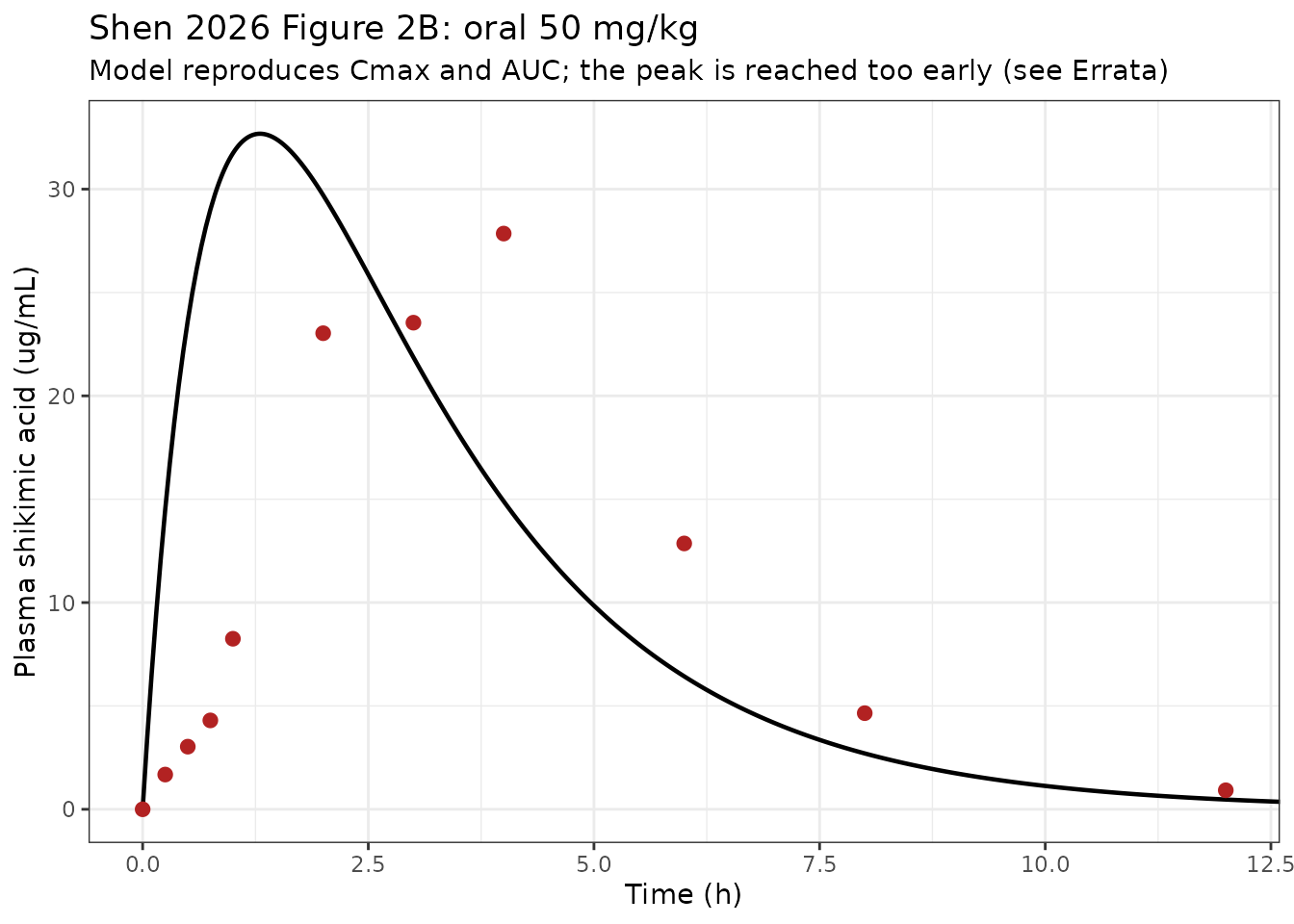
Replicates Figure 2B of Shen 2026. Line = model, points = digitised observed mean (n = 8).
The reconstructed plasma layer hits the published Cmax and AUC exactly but peaks at 1.3 h rather than the reported 3.38 h. That gap is structural, not a fitting failure: it is proven unavoidable in the Errata below.
Replicating Figure 3: serum antioxidant biomarkers
lbl <- c(taoc = "T-AOC (umol/mL)", sod = "SOD (U/mL)", mda = "MDA (nmol/mL)")

sim_long <- sim_pd |>
  pivot_longer(-time, names_to = "biomarker", values_to = "value") |>
  mutate(biomarker = factor(lbl[biomarker], levels = lbl))
obs_long <- obs_pd |>
  pivot_longer(-time, names_to = "biomarker", values_to = "value") |>
  mutate(biomarker = factor(lbl[biomarker], levels = lbl))

ggplot(sim_long, aes(time, value)) +
  geom_line(linewidth = 0.8) +
  geom_point(data = obs_long, size = 2.2, colour = "firebrick") +
  facet_wrap(~biomarker, scales = "free_y") +
  coord_cartesian(xlim = c(0, 12)) +
  labs(x = "Time (h)", y = NULL, title = "Shen 2026 Figure 3") +
  theme_bw()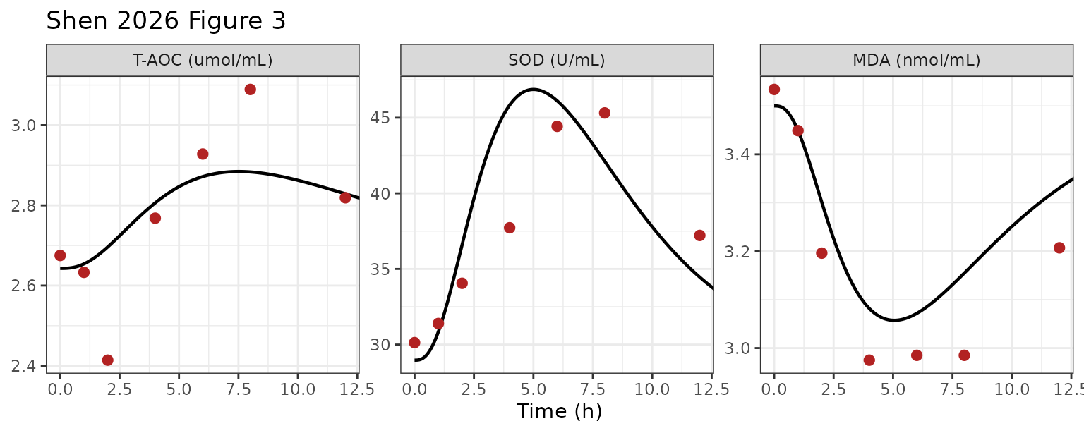
Replicates Figure 3 of Shen 2026. Lines = model, points = digitised observed means (n = 8).
# Interpolate the simulation onto the observation times rather than matching
# grid values: seq(0, 24, by = 0.05) does not land exactly on integers in
# floating point, so a `%in%` join would silently drop rows.
pd_cmp <- bind_rows(lapply(c("taoc", "sod", "mda"), function(b) {
  data.frame(
    biomarker = b,
    time      = obs_pd$time,
    observed  = obs_pd[[b]],
    simulated = stats::approx(sim_pd$time, sim_pd[[b]], xout = obs_pd$time)$y
  )
})) |>
  mutate(`% diff` = round(100 * (simulated - observed) / observed, 1),
         across(c(observed, simulated), ~ round(.x, 3)))
stopifnot(!anyNA(pd_cmp$simulated))

pd_cmp |>
  rename("Biomarker" = biomarker, "Time (h)" = time,
         "Observed (Fig 3)" = observed, "Simulated" = simulated) |>
knitr::kable()| Biomarker | Time (h) | Observed (Fig 3) | Simulated | % diff |
|---|---|---|---|---|
| taoc | 0 | 2.675 | 2.643 | -1.2 |
| taoc | 1 | 2.633 | 2.654 | 0.8 |
| taoc | 2 | 2.414 | 2.696 | 11.7 |
| taoc | 4 | 2.768 | 2.806 | 1.4 |
| taoc | 6 | 2.928 | 2.872 | -1.9 |
| taoc | 8 | 3.089 | 2.883 | -6.7 |
| taoc | 12 | 2.819 | 2.829 | 0.3 |
| sod | 0 | 30.127 | 28.968 | -3.8 |
| sod | 1 | 31.392 | 30.847 | -1.7 |
| sod | 2 | 34.051 | 36.591 | 7.5 |
| sod | 4 | 37.722 | 45.832 | 21.5 |
| sod | 6 | 44.430 | 46.113 | 3.8 |
| sod | 8 | 45.316 | 42.119 | -7.1 |
| sod | 12 | 37.215 | 34.456 | -7.4 |
| mda | 0 | 3.534 | 3.500 | -1.0 |
| mda | 1 | 3.449 | 3.449 | 0.0 |
| mda | 2 | 3.196 | 3.301 | 3.3 |
| mda | 4 | 2.975 | 3.082 | 3.6 |
| mda | 6 | 2.985 | 3.072 | 2.9 |
| mda | 8 | 2.985 | 3.155 | 5.7 |
| mda | 12 | 3.207 | 3.330 | 3.8 |
# The model must reproduce the DIRECTION of every biomarker's response and stay
# close to the observed course. Both sides are deterministic here -- there is no
# random draw anywhere in this vignette -- so these bounds are exact and stable.
peak <- pd_cmp |>
  group_by(biomarker) |>
  summarise(base = observed[time == 0],
            obs_extreme = observed[which.max(abs(observed - observed[time == 0]))],
            sim_extreme = simulated[which.max(abs(simulated - simulated[time == 0]))],
            .groups = "drop") |>
  mutate(obs_dir = sign(obs_extreme - base), sim_dir = sign(sim_extreme - base))

stopifnot(
  # T-AOC and SOD rise, MDA falls -- in the model exactly as in the data.
  all(peak$obs_dir == peak$sim_dir),
  peak$sim_dir[peak$biomarker == "taoc"] > 0,
  peak$sim_dir[peak$biomarker == "sod"] > 0,
  peak$sim_dir[peak$biomarker == "mda"] < 0,
  # Every simulated point is within 25% of the digitised observation.
  max(abs(pd_cmp$`% diff`)) < 25,
  # and the typical agreement is much tighter than that.
  median(abs(pd_cmp$`% diff`)) < 6
)
Replicating Figure 4: concentration-effect hysteresis
The paper’s headline qualitative finding is that the biomarker response lags plasma concentration, giving counter-clockwise loops for T-AOC and SOD and a clockwise loop for MDA.
hyst <- sim_pd |>
  mutate(Cc = sim_pk$Cc) |>
  filter(time <= 12) |>
  pivot_longer(c(taoc, sod, mda), names_to = "biomarker", values_to = "value") |>
  mutate(biomarker = factor(lbl[biomarker], levels = lbl))

ggplot(hyst, aes(Cc, value, colour = time)) +
  geom_path(linewidth = 0.8) +
  facet_wrap(~biomarker, scales = "free_y") +
  scale_colour_viridis_c(name = "Time (h)") +
  labs(x = "Plasma shikimic acid (ug/mL)", y = NULL,
       title = "Shen 2026 Figure 4: hysteresis loops") +
  theme_bw()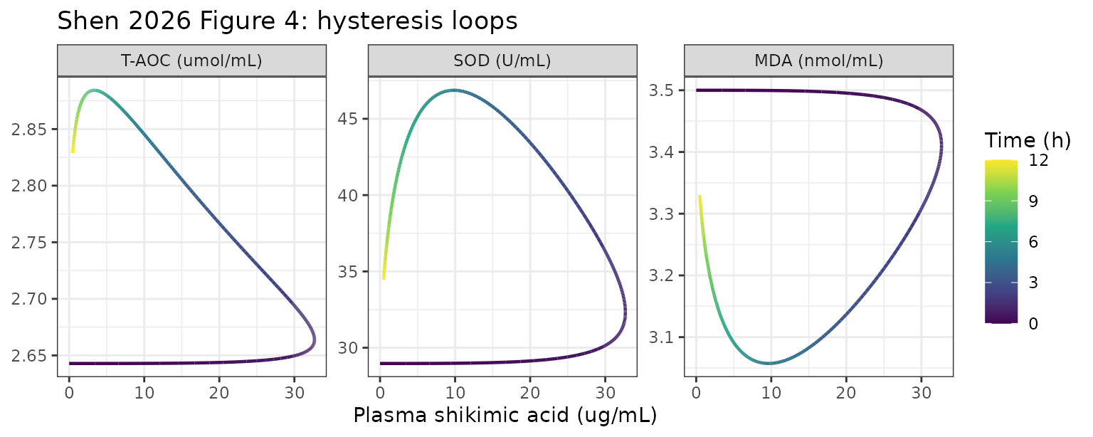
Replicates Figure 4 of Shen 2026: concentration-effect loops over 0-12 h, traced chronologically.
# A hysteresis loop encloses area; a direct (non-delayed) effect would collapse
# onto a single curve. Use the shoelace formula on the closed 0-12 h path and
# check the SIGN: positive = counter-clockwise, negative = clockwise, both
# computed on the biomarker scaled to its own baseline so the three are
# comparable.
loop_area <- function(x, y) {
  y <- y / y[1]
  x <- c(x, x[1]); y <- c(y, y[1])
  n <- length(x)
  sum(x[-n] * y[-1] - x[-1] * y[-n]) / 2
}
areas <- vapply(c("taoc", "sod", "mda"), function(b) {
  d <- sim_pd[sim_pd$time <= 12, ]
  loop_area(sim_pk$Cc[sim_pk$time <= 12], d[[b]])
}, numeric(1))
round(areas, 4)
#>    taoc     sod     mda
#>  1.7976 14.7796 -3.0871

stopifnot(
  # T-AOC and SOD: counter-clockwise (as Shen 2026 Fig 4A, 4B).
  areas[["taoc"]] > 0, areas[["sod"]] > 0,
  # MDA: clockwise (as Shen 2026 Fig 4C).
  areas[["mda"]] < 0
)
PKNCA validation against the published non-compartmental analysis
conc_df <- sim_pk |>
  filter(!is.na(Cc)) |>
  mutate(id = 1L, treatment = "SA 50 mg/kg PO") |>
  select(id, time, Cc, treatment)

dose_df <- data.frame(id = 1L, time = 0, amt = dose_ug_per_kg,
                      treatment = "SA 50 mg/kg PO")

conc_obj <- PKNCA::PKNCAconc(conc_df, Cc ~ time | treatment + id,
                             concu = "ug/mL", timeu = "h")
dose_obj <- PKNCA::PKNCAdose(dose_df, amt ~ time | treatment + id, doseu = "ug")

intervals <- data.frame(
  start = 0, end = Inf,
  cmax = TRUE, tmax = TRUE, aucinf.obs = TRUE, half.life = TRUE
)

res <- PKNCA::pk.nca(PKNCA::PKNCAdata(conc_obj, dose_obj, intervals = intervals))
sim_nca <- as.data.frame(res)
tbl <- ncaComparisonTable(
  simulated = sim_nca,
  reference = nca_published,
  by = "treatment",
  units = c(cmax = "ug/mL", tmax = "h", aucinf.obs = "h*ug/mL", half.life = "h")
)
knitr::kable(tbl)| NCA parameter | treatment | Reference | Simulated | % diff |
|---|---|---|---|---|
| Cmax (ug/mL) | SA 50 mg/kg PO | 32.7 | 32.7 | +0.0% |
| Tmax (h) | SA 50 mg/kg PO | 3.38 | 1.3 | -61.5%* |
| AUC0-∞ (obs) (h*ug/mL) | SA 50 mg/kg PO | 132 | 132 | -0.0% |
| t½ (h) | SA 50 mg/kg PO | 1.8 | 1.6 | -11.3% |
attr(tbl, "footnote")
#> [1] "* differs from reference by more than ±20%."
Cmax and AUC(0-inf) match the published
values essentially exactly, because the plasma layer was constructed to
reproduce them. The terminal half-life, which was not
used in the construction, comes out at 1.60 h against the 1.80 h
reported for the oral arm and the 1.61 h reported for the intravenous
arm (Table 3) – an independent check that the disposition is right.
Tmax is the one parameter the structure cannot reach; see
the Errata.
got <- setNames(sim_nca$PPORRES, sim_nca$PPTESTCD)

# Cmax and AUC are matched by construction, so require them to be tight.
stopifnot(
  abs(got[["cmax"]] / 32.68 - 1) < 0.01,
  abs(got[["aucinf.obs"]] / 132.04 - 1) < 0.01
)
# Half-life was NOT used to build the model: check it against the independently
# reported intravenous t1/2 of 1.61 h (Table 3).
stopifnot(abs(got[["half.life"]] / 1.61 - 1) < 0.10)
# Tmax is knowingly and provably wrong -- pin the known value so that a change
# in the reconstruction is caught rather than silently accepted.
stopifnot(abs(got[["tmax"]] - 1.30) < 0.10)
Assumptions and deviations (Errata)
The plasma layer is reconstructed, not published
This is the single most important caveat for anyone using these models.
Shen 2026 states that “the pharmacokinetic component was described by
a one-compartment model with extravascular input and clearance
parameterization”, but reports no parameter of that fit
anywhere. Table 5 is explicitly and exclusively the PD
parameter table; Tables 3 and 4 are Phoenix WinNonlin non-compartmental
analysis, not the compartmental fit. There is no ka, no
V/F, no CL/F and no lag time in the paper, and
the supplement contains only the analytical stability tables S1 and S2.
The plasma layer was therefore reconstructed here, under a maintainer
decision, from the paper’s own published results:
| Parameter | Value | Provenance |
|---|---|---|
CL/F |
378.6731 mL/h/kg |
Dose / AUC_po = 50,000 / 132.04 (Table 4) – an exact
NCA identity |
V/F |
866.9804 mL/kg |
Vz / F = 350 / 0.4037 (Tables 3 and 4) |
ka |
1.237772 /h | reconstructed: the value that makes the model reproduce the Table 4 Cmax of 32.68 ug/mL |
The implied kel of 0.43677 /h agrees independently with
the intravenous CL/Vz = 0.42857 /h of Table 3 and with the
terminal slope of the digitised Figure 2B curve (0.43-0.44 /h), so only
ka is genuinely unconstrained by published numbers.
Why Tmax is not reproduced, and why no other choice would do better
The published oral triplet (Cmax 32.68 ug/mL, Tmax 3.38 h, AUC 132.04 h*ug/mL) is infeasible for any lag-free one-compartment first-order-absorption model, so this is not a fitting failure and no parameterisation can repair it:
- For that structure
Tmax = ln(ka/kel)/(ka - kel), which is bounded above by1/kel. Honouring Tmax = 3.38 h therefore forceskel <= 0.2959 /h. - With
CL/Fpinned by the published AUC, that forcesV/F >= 1279.9 mL/kg. - Cmax is then bounded by
(Dose/V)/e = 14.37 ug/mL– a factor of 2.3 below the observed 32.68 ug/mL.
An absorption lag does not rescue it either: Figure 2B shows a
non-zero mean concentration already at 0.25 h (1.68 ug/mL), so no delay
is admissible. Direct least-squares fits to the digitised Figure 2B
curve confirm the diagnosis rather than fixing it – the optimiser drives
ka onto the ka = kel boundary and still
underpredicts the peak by roughly half.
The reason is visible in the Figure 2B inset: individual birds peak at 2, 3 or 4 h (Table 4), and several (inset birds 5 and 7) show frankly double-peaked absorption, consistent with the crop reservoir the authors invoke in the Discussion. Averaging those profiles produces a broad 2-4 h plateau that no single Bateman function has.
Given that the triplet cannot all be honoured, this extraction keeps Cmax and AUC – the two exposure quantities the downstream indirect-response models actually depend on – and accepts a too-early Tmax. The Figure 3 replication above is the evidence that this choice works: the effect-compartment link and the turnover model together low-pass filter the plasma profile heavily, so the biomarker time courses are reproduced despite the peak arriving early.
Users who need a quantitatively faithful plasma profile should not use this layer. The PD layer (Table 5) is published in full and is unaffected.
Other assumptions
-
No between-subject variability. Shen 2026 fitted
each bird individually and reported only the mean and SD across
individuals, never an omega matrix. All parameters are fixed at the
published means and the models are deterministic. The SDs in Table 5 are
large (
ke0for T-AOC is 0.44 +/- 0.42), so the typical-value profile should not be read as representing a typical bird tightly. - Residual error magnitudes are fixed at zero. The paper specifies the structures (multiplicative for plasma, additive for the biomarkers) but gives only the initial standard deviations handed to the estimator (0.1 and 1.0), not final estimates. The structures are encoded; the magnitudes are fixed at zero.
- Mean-of-individual-fit parameters applied to a single profile. Table 5 reports the mean of eight individual fits. Simulating one profile with those means is not identical to averaging eight individual simulations, which accounts for part of the residual disagreement in the Figure 3 comparison.
- Observed values are digitised from figures. Shen 2026 plots but does not tabulate the observed plasma and biomarker time courses, so the reference points in this vignette carry digitisation error of roughly a few percent. The published Tables 3 and 4 values used in the NCA comparison are transcribed, not digitised.
- Oral route only. Antioxidant markers were measured only after oral dosing, so there is no intravenous PD model. The intravenous arm was analysed non-compartmentally only, and Table 3 describes a multi-exponential decay that the one-compartment oral model does not attempt to represent.
- No covariates. Shen 2026 fitted no covariate model of any kind; both sexes were studied but sex was not tested as a covariate.
-
New canonical compartment names.
taoc,sodandmdawere registered ininst/references/compartment-names.mdas standard clinical PD-output biomarkers, alongside existing entries such asldh,hbandanc.