Model and source
- Citation: Le KN, Gibiansky L, van Lookeren Campagne M, Good J, Davancaze T, Loyet KM, Morimoto A, Strauss EC, Jin JY. Population Pharmacokinetics and Pharmacodynamics of Lampalizumab Administered Intravitreally to Patients With Geographic Atrophy. CPT Pharmacometrics Syst Pharmacol. 2015;4(10):595-604. doi:[10.1002/psp4.12031](https://doi.org/10.1002/psp4.12031).
- Description: Combined ocular-serum target-mediated drug-disposition (TMDD) model with quasi-steady-state binding approximation for intravitreally administered lampalizumab (anti-complement factor D Fab) and total complement factor D (CFD) in adults with geographic atrophy (GA) secondary to age-related macular degeneration (AMD).
- Modality: Humanized antibody-binding fragment (Fab) of an anti-CFD monoclonal antibody (Fab ~ 48 kDa); administered intravitreally (ITV); developed by Genentech / Roche.
- Article (open access): https://doi.org/10.1002/psp4.12031
Population
The model was developed from the integrated PK / PD dataset of two Genentech-sponsored clinical studies in patients with geographic atrophy (Le 2015 Methods - Study design, Table 1 paragraph 1):
- CFD4711g (NCT00973011, phase Ia single-ascending-dose): 18 patients (3 per dose level) received a single ITV administration of lampalizumab at 0.1, 0.5, 1, 2, 5, or 10 mg in the study eye. Serum lampalizumab was sampled at screening, day 1, 7, 14, and 30 post-dose.
- CFD4870g MAHALO (NCT01229215, phase Ib/II): an open-label safety run-in (n=14) of >=3 monthly ITV doses of 10 mg followed by an 18-month randomized phase II in which 129 patients received either 10 mg q4w, 10 mg q8w, or sham. Serum trough was sampled at screening, monthly months 1-3, and at months 1, 2, 3, 6, 9, 12, 15, and 18. Aqueous humor lampalizumab and total CFD were sampled at screening, month 6 pre-dose, and month 12 pre-dose (n=12 ocular).
The combined model dataset comprises 117 patients
with 697 quantifiable serum lampalizumab
concentrations, 24 quantifiable aqueous humor
lampalizumab concentrations, and 62 quantifiable
aqueous humor total CFD concentrations from a 21-patient ocular
subset (Le 2015 Results - Serum pharmacokinetics / Ocular
pharmacokinetics). The lower limits of quantitation were 350 pg/mL
(serum), 30 ng/mL (aqueous lampalizumab), and 5 ng/mL (aqueous CFD). The
Table 1 reference patient is an 80-year-old male; per-subject weight,
race, and exact age distributions reside in the source paper’s
Supplemental Table 1, which was not bundled with the main PDF and is
therefore not reproduced in population metadata.
The packaged population metadata is available
programmatically via
readModelDb("Le_2015_lampalizumab")$population.
Source trace
Every parameter is annotated in the model file
(inst/modeldb/specificDrugs/Le_2015_lampalizumab.R) with an
in-file comment pointing to Le 2015 Table 1 row by row. The table below
collects the equations and parameters in one place for reviewers.
| Equation / parameter | Value (typical, 80-yr-old male) | Source location |
|---|---|---|
d/dt(depot) (lampalizumab in vitreous, mg) |
n/a | Le 2015 Eq. 1, p.596 |
d/dt(total_target) (total CFD in vitreous, mg/L =
ug/mL) |
n/a | Le 2015 Eq. 2, p.596 |
d/dt(central) (lampalizumab in serum, mg) |
n/a | Le 2015 Eq. 3, p.596 |
Cunbound (QSS algebra) |
n/a | Le 2015 Eq. 4, p.596 |
CAQ = CVITR / kAQ (aqueous humor lampalizumab,
mg/L) |
n/a | Le 2015 Eq. 5, p.596 |
RAQ = total_target / kTAQ (aqueous humor total CFD,
mg/L) |
n/a | Le 2015 Eq. 6, p.596 |
kTAQ = kAQ * kA |
29.0 | Le 2015 Eq. 7, p.596; Results p.598 |
kout (ocular drug elimination rate, 1/day) |
0.117 | Le 2015 Table 1, row 1 |
koutC (ocular complex elimination rate, 1/day) |
0.135 | Le 2015 Table 1, row 2 |
kinT (ocular target influx/synthesis, ug/mL/day) |
0.364 | Le 2015 Table 1, row 3 (text Discussion cites 0.32 ug/mL/day) |
kA (drug:target MW/assay correction factor,
unitless) |
2.23 | Le 2015 Table 1, row 4 |
VVITR (vitreous volume, L) |
0.00309 (3.09 mL) | Le 2015 Table 1, row 5 |
koutT (ocular target degradation rate, 1/day) |
0.27 | Le 2015 Table 1, row 6 |
kAQ (vitreous-to-aqueous partition of drug,
unitless) |
13.0 | Le 2015 Table 1, row 7 |
Vc (serum volume, L) |
2.41 (2410 mL) | Le 2015 Table 1, row 8 |
k (systemic elimination rate, 1/day) |
1.89 | Le 2015 Table 1, row 9 |
Kss (QSS binding constant, mg/L) – FIXED |
0.00096 (~20 pM) | Le 2015 Table 1, row 10 (footnote d: fixed) |
e_age_kout (power exponent for AGE/80 on kout) |
-0.770 | Le 2015 Table 1, Covariates block |
e_age_k (power exponent for AGE/80 on k) |
-1.63 | Le 2015 Table 1, Covariates block |
e_sexf_k (multiplier for female sex on k; ref =
male) |
0.739 | Le 2015 Table 1, Covariates block |
IIV CV% on kout / kA / k
|
27.3 / 59.1 / 27.5 | Le 2015 Table 1, Variability block |
| Proportional residual SD: serum / aqueous | 0.329 / 0.258 | Le 2015 Table 1, Variability block |
The pre-dose initial condition
total_target(0) = kinT / koutT = 0.364 / 0.27 = 1.35 mg/L
(~1.35 ug/mL) is the analytical steady state of Eq. 2 in the absence of
drug (d/dt(total_target) = 0 when
Cunbound = 0).
Errata note
A PubMed search (May 2026) for
10.1002/psp4.12031 AND erratum returned no records. No
errata or corrigenda were identified at the time of extraction.
Virtual cohort
The model’s structural parameters are calibrated to a typical 80-year-old male (Le 2015 Table 1 footnote a). The virtual cohort below samples ages spanning a plausible GA population (60-90 years) and a roughly balanced sex distribution so the covariate effects are exercised. Original observed data are not publicly available.
set.seed(20260512)

n_subj <- 60
cohort <- tibble::tibble(
  id   = seq_len(n_subj),
  AGE  = pmin(pmax(round(rnorm(n_subj, mean = 80, sd = 7)), 60), 95),
  SEXF = rbinom(n_subj, size = 1, prob = 0.55)
)
Three dosing regimens are simulated for the figure-replication panel:
10 mg ITV every 4 weeks (q4w), every 6 weeks (q6w), and every 8 weeks
(q8w), each for 16 weeks of dosing followed by a 4-week tail. Each
regimen is given its own disjoint id block (per
vignette-template.md’s multi-cohort guidance) so
rxSolve does not silently merge subjects across regimens.
The observation grid is dense in the first week (where vitreous-to-serum
egress dominates) and coarse afterward to keep the simulation under the
pkgdown vignette time budget.
horizon_days <- 16 * 7 + 28          # 16 wk dosing + 4 wk tail
obs_times    <- sort(unique(c(
  0, seq(0.25, 7, by = 0.5),         # dense first week
  seq(10, horizon_days, by = 3)      # every 3 days thereafter
)))

dose_times <- list(
  "q4w" = seq(0, by = 28, length.out = 5),
  "q6w" = seq(0, by = 42, length.out = 3),
  "q8w" = seq(0, by = 56, length.out = 2)
)

build_regimen <- function(pop, regimen_label, dose_days, id_offset) {
  pop_off <- pop |>
    dplyr::mutate(id = id + id_offset, regimen = regimen_label)

  d_dose <- pop_off |>
    tidyr::crossing(time = dose_days) |>
    dplyr::mutate(amt = 10, evid = 1L, cmt = "depot")

  d_obs_cc <- pop_off |>
    tidyr::crossing(time = obs_times) |>
    dplyr::mutate(amt = 0, evid = 0L, cmt = "Cc")

  d_obs_caq <- pop_off |>
    tidyr::crossing(time = obs_times) |>
    dplyr::mutate(amt = 0, evid = 0L, cmt = "CAQ")

  d_obs_raq <- pop_off |>
    tidyr::crossing(time = obs_times) |>
    dplyr::mutate(amt = 0, evid = 0L, cmt = "RAQ")

  dplyr::bind_rows(d_dose, d_obs_cc, d_obs_caq, d_obs_raq) |>
    dplyr::arrange(id, time, dplyr::desc(evid)) |>
    as.data.frame()
}

events <- dplyr::bind_rows(
  build_regimen(cohort, "q4w", dose_times[["q4w"]], id_offset =     0L),
  build_regimen(cohort, "q6w", dose_times[["q6w"]], id_offset = 1000L),
  build_regimen(cohort, "q8w", dose_times[["q8w"]], id_offset = 2000L)
)

stopifnot(!anyDuplicated(unique(events[, c("id", "time", "evid", "cmt")])))
Simulation
Two model objects are used:
-
mod– the packaged model with between-subject variability, for prediction intervals. -
mod_typ– the same model with random effects zeroed (rxode2::zeroRe) for typical-value curves.
mod     <- rxode2::rxode2(readModelDb("Le_2015_lampalizumab"))
#> ℹ parameter labels from comments will be replaced by 'label()'
mod_typ <- mod |> rxode2::zeroRe()

sim <- rxode2::rxSolve(mod, events = events,
                       keep = c("regimen", "AGE", "SEXF"),
                       returnType = "data.frame")

# Endpoint compartment numbering: depot=1, total_target=2, central=3,
# Cc=4, CAQ=5, RAQ=6.
sim_cc  <- sim |> dplyr::filter(CMT == 4)
sim_caq <- sim |> dplyr::filter(CMT == 5)
sim_raq <- sim |> dplyr::filter(CMT == 6)
Replicate published figures
Vitreous (aqueous proxy) lampalizumab concentration (replicates Figure 4a of Le 2015)
Le 2015 Figure 4a plots simulated vitreous lampalizumab concentration
over time for the three 10-mg regimens (q4w, q6w, q8w) with the 5th to
95th prediction band. We approximate the vitreous concentration as
CAQ * kAQ (paper’s Eq. 5 inverted; kAQ = 13),
restoring vitreous units from the aqueous-humor proxy. The relevant
biology is the trough relative to the alternative-pathway IC50 of 0.2
ug/mL = 0.2 mg/L (paper text Discussion: “the 5th percentile of vitreous
humor Cmin values for 10 mg per eye were above the median inhibitory
concentration (IC50) (0.2 ug/mL or 4 nM)”), shown as a dashed reference
line.
kAQ_nominal <- 13

sim_vitreous <- sim_caq |>
  dplyr::mutate(CVITR = CAQ * kAQ_nominal) |>
  dplyr::group_by(regimen, time) |>
  dplyr::summarise(
    Q05 = quantile(CVITR, 0.05, na.rm = TRUE),
    Q50 = quantile(CVITR, 0.50, na.rm = TRUE),
    Q95 = quantile(CVITR, 0.95, na.rm = TRUE),
    .groups = "drop"
  )

ggplot(sim_vitreous, aes(time, Q50, colour = regimen, fill = regimen)) +
  geom_ribbon(aes(ymin = Q05, ymax = Q95), alpha = 0.18, colour = NA) +
  geom_line(linewidth = 0.9) +
  geom_hline(yintercept = 0.2, linetype = "dashed", colour = "grey40") +
  scale_y_log10() +
  labs(
    x = "Time since first dose (days)",
    y = "Vitreous lampalizumab concentration (mg/L = ug/mL)",
    title = "Replicates Le 2015 Figure 4a (vitreous lampalizumab, three 10-mg regimens)",
    subtitle = "Median and 5th-95th prediction interval. Dashed line = alternative-complement IC50 (0.2 ug/mL).",
    colour = "Regimen", fill = "Regimen"
  ) +
  theme_bw()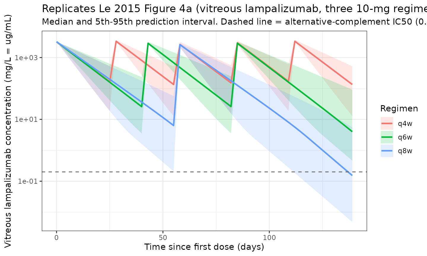
Serum lampalizumab concentration (replicates Figure 4b of Le 2015)
Le 2015 Figure 4b shows the corresponding serum profile. The paper narrative emphasises that systemic Cmax stays well below the 2 ug/mL threshold required to inhibit systemic alternative-complement activity (reference line below).
sim_serum <- sim_cc |>
  dplyr::group_by(regimen, time) |>
  dplyr::summarise(
    Q05 = quantile(Cc, 0.05, na.rm = TRUE),
    Q50 = quantile(Cc, 0.50, na.rm = TRUE),
    Q95 = quantile(Cc, 0.95, na.rm = TRUE),
    .groups = "drop"
  )

ggplot(sim_serum, aes(time, Q50, colour = regimen, fill = regimen)) +
  geom_ribbon(aes(ymin = Q05, ymax = Q95), alpha = 0.18, colour = NA) +
  geom_line(linewidth = 0.9) +
  geom_hline(yintercept = 2, linetype = "dashed", colour = "grey40") +
  scale_y_log10(limits = c(1e-4, 5)) +
  labs(
    x = "Time since first dose (days)",
    y = "Serum lampalizumab concentration (mg/L = ug/mL)",
    title = "Replicates Le 2015 Figure 4b (serum lampalizumab, three 10-mg regimens)",
    subtitle = "Median and 5th-95th prediction interval. Dashed line = systemic complement-inhibition threshold (2 ug/mL).",
    colour = "Regimen", fill = "Regimen"
  ) +
  theme_bw()
#> Warning in scale_y_log10(limits = c(1e-04, 5)): log-10 transformation introduced infinite values.
#> log-10 transformation introduced infinite values.
#> log-10 transformation introduced infinite values.
#> log-10 transformation introduced infinite values.
#> Warning: Removed 21 rows containing missing values or values outside the scale range
#> (`geom_ribbon()`).
#> Warning: Removed 6 rows containing missing values or values outside the scale range
#> (`geom_line()`).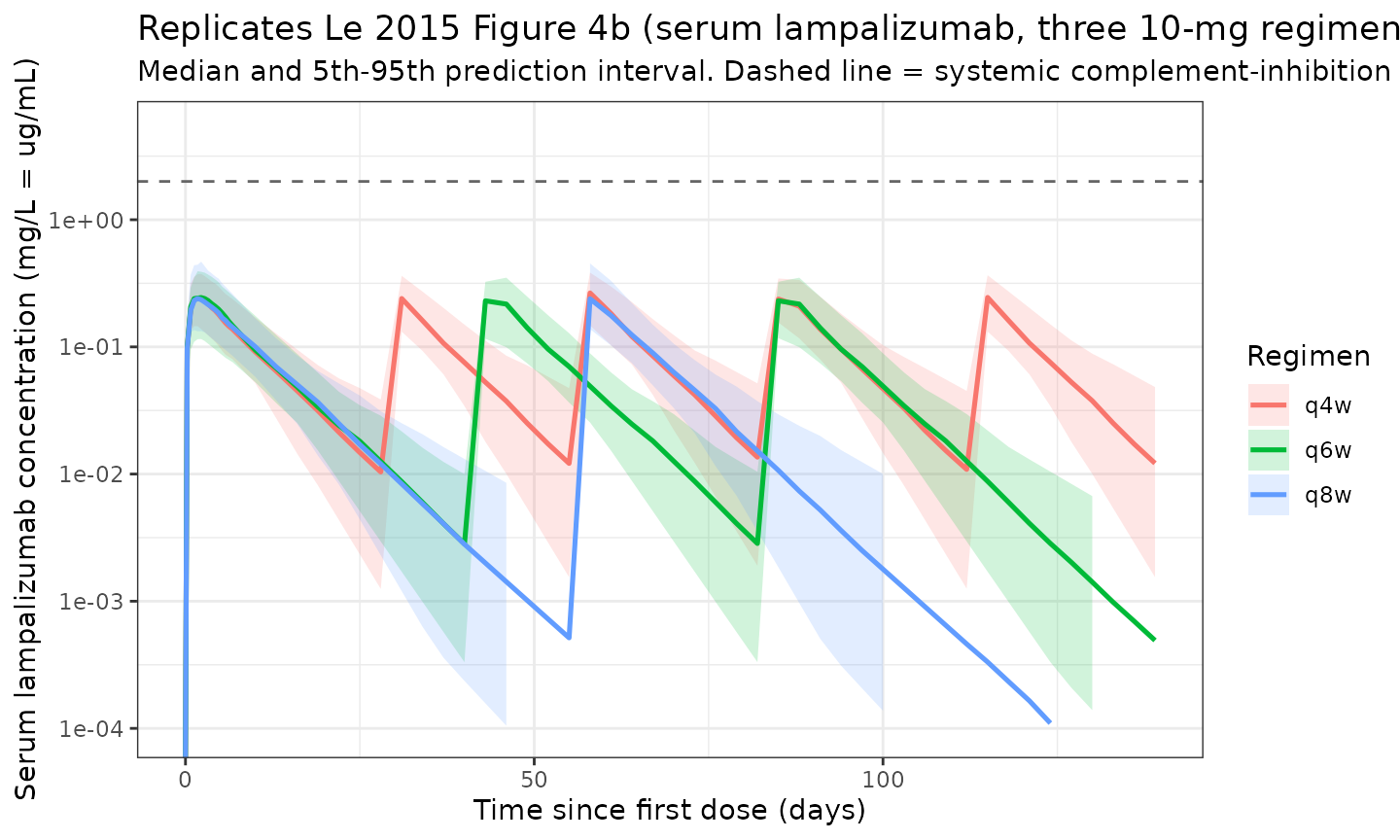
Free target ratio in vitreous (replicates Figure 6 of Le 2015)
Le 2015 Figure 6 plots the simulated free CFD-to-baseline ratio (FTR) in the vitreous over time for the three regimens, illustrating near-complete target suppression at day 60 post-dose. With the QSS algebra,
free CFD concentration in vitreous = R_total * Kss / (Kss + Cunbound) FTR = free CFD / baseline target = (R_total * Kss / (Kss + Cunbound)) / (kinT / koutT)
is derived directly from the model’s internal
total_target and Cunbound states (both
available in sim).
ftr_typ_events <- events |>
  dplyr::filter(id %in% c(1L, 1001L, 2001L))   # one typical subject per regimen

sim_typ <- rxode2::rxSolve(mod_typ, events = ftr_typ_events,
                           keep = c("regimen"),
                           returnType = "data.frame")
#> ℹ omega/sigma items treated as zero: 'etalkout', 'etalkA', 'etalk'
#> Warning: multi-subject simulation without without 'omega'

kinT_val  <- 0.364
koutT_val <- 0.27
Kss_val   <- 0.96e-3
R_baseline <- kinT_val / koutT_val

sim_ftr <- sim_typ |>
  dplyr::filter(CMT == 5) |>                        # any output row is fine; pick CAQ rows
  dplyr::mutate(
    free_target = total_target * Kss_val / (Kss_val + Cunbound),
    FTR         = free_target / R_baseline
  )

ggplot(sim_ftr, aes(time, FTR, colour = regimen)) +
  geom_line(linewidth = 0.9) +
  scale_y_continuous(limits = c(0, 1.2)) +
  labs(
    x = "Time since first dose (days)",
    y = "Free CFD / baseline CFD (vitreous)",
    title = "Replicates Le 2015 Figure 6 (vitreous free-target ratio, typical subject)",
    subtitle = "Typical 80-yr-old male (etas = 0); near-complete suppression sustained through dosing interval.",
    colour = "Regimen"
  ) +
  theme_bw()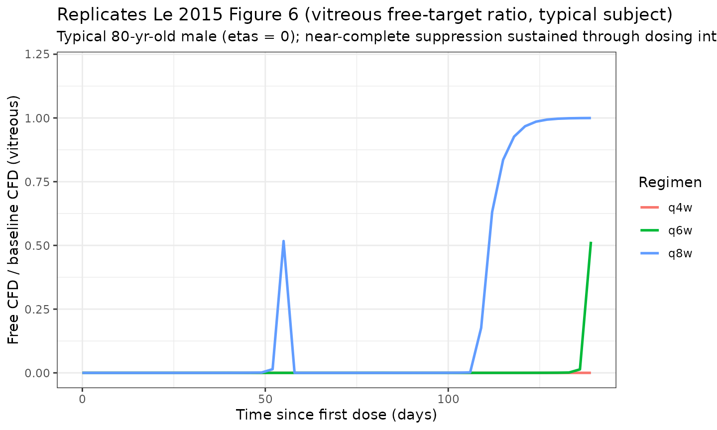
Key quantitative checks against Le 2015 Results / Discussion
The Le 2015 supplement (Supplemental Table 3) reports per-regimen Cmax / Cmin / AUC for vitreous and serum, but is not bundled with the main PDF; the paper’s main-text quantitative claims below are reproducible from the simulation above.
single_dose_events <- cohort |>
  dplyr::slice(1L) |>
  dplyr::mutate(time = 0, amt = 10, evid = 1L, cmt = "depot") |>
  dplyr::bind_rows(
    tidyr::crossing(cohort |> dplyr::slice(1L), time = obs_times) |>
      dplyr::mutate(amt = 0, evid = 0L, cmt = "Cc"),
    tidyr::crossing(cohort |> dplyr::slice(1L), time = obs_times) |>
      dplyr::mutate(amt = 0, evid = 0L, cmt = "CAQ"),
    tidyr::crossing(cohort |> dplyr::slice(1L), time = obs_times) |>
      dplyr::mutate(amt = 0, evid = 0L, cmt = "RAQ")
  ) |>
  dplyr::arrange(id, time, dplyr::desc(evid)) |>
  as.data.frame()

sim_typ_single <- rxode2::rxSolve(mod_typ, events = single_dose_events,
                                  returnType = "data.frame")
#> ℹ omega/sigma items treated as zero: 'etalkout', 'etalkA', 'etalk'

cc_single  <- sim_typ_single |> dplyr::filter(CMT == 4)
caq_single <- sim_typ_single |> dplyr::filter(CMT == 5)

vitreous_cmax <- max(caq_single$CAQ * kAQ_nominal, na.rm = TRUE)
serum_cmax    <- max(cc_single$Cc, na.rm = TRUE)
ratio_cmax    <- vitreous_cmax / serum_cmax

knitr::kable(
  data.frame(
    Metric = c(
      "Vitreous Cmax (mg/L)",
      "Serum Cmax (mg/L)",
      "Vitreous / Serum Cmax ratio",
      "Ocular elimination t1/2 (days)",
      "True serum elimination t1/2 (days)",
      "Apparent (flip-flop) serum t1/2 (days)"
    ),
    `Simulated value` = c(
      sprintf("%.0f", vitreous_cmax),
      sprintf("%.4f", serum_cmax),
      sprintf("%.0f-fold", ratio_cmax),
      sprintf("%.2f", log(2) / 0.117),
      sprintf("%.3f", log(2) / 1.89),
      "see PKNCA section below"
    ),
    `Le 2015 reported value` = c(
      "n/a (main text uses ratio only)",
      "n/a (main text uses ratio only)",
      "> 11,000-fold (Discussion p.601)",
      "5.9 days (Results p.599)",
      "0.367 days = 9 hours (Discussion p.600)",
      "5.9 days (apparent; flip-flop, Discussion p.601)"
    ),
    check.names = FALSE
  ),
  caption = "Quantitative checks of single 10 mg ITV dose simulation vs Le 2015."
)| Metric | Simulated value | Le 2015 reported value |
|---|---|---|
| Vitreous Cmax (mg/L) | 3236 | n/a (main text uses ratio only) |
| Serum Cmax (mg/L) | 0.2389 | n/a (main text uses ratio only) |
| Vitreous / Serum Cmax ratio | 13547-fold | > 11,000-fold (Discussion p.601) |
| Ocular elimination t1/2 (days) | 5.92 | 5.9 days (Results p.599) |
| True serum elimination t1/2 (days) | 0.367 | 0.367 days = 9 hours (Discussion p.600) |
| Apparent (flip-flop) serum t1/2 (days) | see PKNCA section below | 5.9 days (apparent; flip-flop, Discussion p.601) |
PKNCA validation – serum lampalizumab after a single 10 mg ITV dose
Single-dose NCA on serum lampalizumab is the most directly comparable check: with flip-flop PK the apparent serum half-life equals the ocular elimination half-life of 5.9 days (Le 2015 Discussion: “the flip-flop PK phenomenon enabled the use of systemic half-life following ITV administration as a surrogate for ocular half-life”). The cohort below is the same virtual population as the dosing simulations above, given a single 10-mg ITV dose; PKNCA computes Cmax, Tmax, AUC, and the apparent terminal half-life per subject.
suppressPackageStartupMessages(library(PKNCA))

# Use a smaller PKNCA cohort to keep the vignette inside the pkgdown
# 5-minute time budget; 30 subjects is sufficient for the apparent
# terminal-half-life check that is the headline NCA result.
pknca_cohort <- cohort |>
  dplyr::slice(seq_len(30L)) |>
  dplyr::mutate(regimen = "single_10mg")

pknca_obs_times <- sort(unique(c(0, 0.5, 1, 2, 4, 7, 10, 14, 21, 28, 42, 56)))

d_dose_p <- pknca_cohort |>
  dplyr::mutate(time = 0, amt = 10, evid = 1L, cmt = "depot")

d_obs_p <- pknca_cohort |>
  tidyr::crossing(time = pknca_obs_times) |>
  dplyr::mutate(amt = 0, evid = 0L, cmt = "Cc")

ev_p <- dplyr::bind_rows(d_dose_p, d_obs_p) |>
  dplyr::arrange(id, time, dplyr::desc(evid)) |>
  as.data.frame()

sim_p <- rxode2::rxSolve(mod, events = ev_p,
                         keep = c("regimen"),
                         returnType = "data.frame") |>
  dplyr::filter(CMT == 4)

conc_df <- sim_p |>
  dplyr::filter(!is.na(Cc)) |>
  dplyr::select(id, regimen, time, Cc)

dose_df <- d_dose_p |>
  dplyr::select(id, regimen, time, amt)

conc_obj <- PKNCA::PKNCAconc(conc_df, Cc ~ time | regimen + id,
                             concu = "mg/L", timeu = "day")
dose_obj <- PKNCA::PKNCAdose(dose_df, amt ~ time | regimen + id,
                             doseu = "mg")

intervals <- data.frame(
  start      = 0,
  end        = Inf,
  cmax       = TRUE,
  tmax       = TRUE,
  auclast    = TRUE,
  aucinf.obs = TRUE,
  half.life  = TRUE
)

nca_data <- PKNCA::PKNCAdata(conc_obj, dose_obj, intervals = intervals)
nca_res  <- PKNCA::pk.nca(nca_data)

knitr::kable(summary(nca_res),
caption = "Serum lampalizumab NCA after single 10 mg ITV dose (apparent terminal half-life is the flip-flop ocular t1/2 ~ 5.9 days).")| Interval Start | Interval End | regimen | N | AUClast (day*mg/L) | Cmax (mg/L) | Tmax (day) | Half-life (day) | AUCinf,obs (day*mg/L) |
|---|---|---|---|---|---|---|---|---|
| 0 | Inf | single_10mg | 30 | 2.50 [31.1] | 0.235 [31.9] | 2.00 [1.00, 2.00] | 6.23 [1.19] | 2.51 [31.2] |
The apparent terminal half-life from PKNCA is the flip-flop half-life dictated by the slower ocular elimination (kout = 0.117/day, t1/2 ~ 5.9 days), not the true serum k = 1.89/day (t1/2 ~ 9 hours). This is a load-bearing biological feature of intravitreally administered Fabs (Le 2015 Discussion p.601) – not a model artefact.
Assumptions and deviations
-
Compartment naming. The vitreous (intravitreal
injection site, drug-target binding site, and aqueous-humor observation
source) is encoded as the model’s
depotcompartment, since ITV dosing is extravascular and the source-paper’s vitreous compartment maps cleanly to the canonical depot role. Aqueous humor concentrations are derived algebraically fromdepot / VVITRvia the partition coefficientkAQ, not carried as a separate state. The serum sampling site is the canonicalcentralcompartment. The CFD compartment uses the canonicaltotal_targetname (total free + bound target in the QSS approximation; Gibiansky 2008). No compartment names outside the canonical register are introduced. -
target_totalcarries CONCENTRATION units, not amount. Paper Eq. 2 is written directly in concentration units (mg/L), andkinThas units of mg/L/day. The model preserves the paper’s formulation rather than redundantly multiplying through byVVITR; observed aqueous CFD (RAQ) is derived astotal_target / kTAQ. This is a faithful translation of the source equations and is flagged here because most popPK compartments carry amount units. -
Shared aqueous residual encoded as two parameters.
Le 2015 Table 1 reports a single proportional residual SD (25.8%) for
aqueous-humor measurements (lampalizumab AND CFD combined). nlmixr2’s
residual-error syntax requires one endpoint parameter per output, so the
shared residual is encoded as two parameters (
propSd_CAQ,propSd_RAQ) initialised to the same Table 1 value of 0.258. Re-estimation would treat them as independent; for prediction / simulation they remain numerically identical, so the packaged model reproduces the paper’s residual structure exactly. -
IIV variance scale. Le 2015 Table 1 reports
inter-subject variability as a CV% for the three retained random effects
(
kout27.3%,kA59.1%,k27.5%). Per the source paper’s convention with log-normal etas at these CV magnitudes, the packaged variance of the log-eta is taken asCV^2directly (0.0745, 0.349, 0.0756). The alternative log-normal formomega^2 = log(1 + CV^2)differs by ~10% for the largest CV (0.349 vs 0.323) and is documented here for reviewer transparency. The other parameters were held at 1% CV during backward elimination (Le 2015 Methods p.596) and are not carried as etas in the packaged model. -
Kssis fixed. The QSS binding constant is held at the in-vitro KD value of ~20 pM (= 0.96e-3 mg/L for a 48 kDa Fab, Le 2015 Table 1 footnote d). Wrapped infixed()inini(). -
kinTtable value used (0.364 ug/mL/day). Le 2015 Table 1 reportskinT = 0.364 mg/mL/daywhile the paper’s Discussion (p.600) refers to “0.32 ug/mL/day”. The order-of-magnitude argument that follows (“0.91 ug/day, less than 1% of systemic production rate of 1.33 mg/kg/day”) confirms the table’s unit is ug/mL/day, not mg/mL/day. The minor numerical discrepancy between 0.364 (table) and 0.32 (text) is treated as a paper-text approximation; the Table 1 point estimate is used in the model. - Reference age 80 yr, reference sex male. Le 2015 Table 1 footnote a explicitly anchors the typical parameters to an “80-year-old male patient”; the model preserves this reference point in the covariate-effect equations.
-
Sparse / missing baseline demographics. Per-subject
weight, race, and exact age distributions reside in the paper’s
Supplemental Table 1, which was not bundled with the on-disk PDF.
population$weight_range,race_ethnicity, andsex_female_pctare thereforeNULLrather than guessed. Any reader needing the demographic distribution should consult the paper’s supplement directly. - Original concentration data not publicly available. All validation in this vignette uses model-derived simulations compared back to the paper’s main-text quantitative claims (vitreous-to-serum ratio > 11,000-fold; ocular t1/2 ~ 5.9 days; flip-flop apparent serum t1/2 ~ 5.9 days; near-complete vitreous target suppression at day 60). Numerical NCA values from Supplemental Table 3 are not reproduced because the supplement was not on disk.
-
No errata identified. A PubMed search for the DOI
plus
erratum(May 2026) returned no records. No errata or corrigenda were applied.