Luvometinib (Tan 2023)

Model and source

• Citation: Tan Y., Cui A., Qian L., Li C., Wu Z., Yang Y., Han P., Huang X., Diao L. (2023). Population pharmacokinetics of FCN-159, a MEK1/2 inhibitor, in adult patients with advanced melanoma and neurofibromatosis type 1 (NF1) and model informed dosing recommendations for NF1 pediatrics. Frontiers in Pharmacology 14:1101991. doi:10.3389/fphar.2023.1101991.
• Description: Two-compartment population PK model for oral luvometinib (FCN-159), a MEK1/2 inhibitor, in 45 Chinese adults with advanced NRAS-aberrant melanoma or neurofibromatosis type 1 (NF1) pooled from two phase I studies. First-order absorption with an absorption lag time and linear elimination. Body surface area enters all four disposition parameters as an estimated power function centered at 1.66 m^2; total serum protein scales the central volume, female sex enlarges the peripheral volume, and relative bioavailability is 1.29-fold higher in NF1 than in melanoma. Log-normal between-subject variability on CL/F, Vc/F, Q/F and Vp/F with a proportional residual error.
• Article: https://doi.org/10.3389/fphar.2023.1101991 (open access)

The paper names the drug by its development code, FCN-159. Its international nonproprietary name is luvometinib (approved in China in 2025), which is the name used for the model file.

Population

The model was fit to 1030 plasma concentrations from 45 Chinese adults in two phase I studies, both dosing luvometinib tablets once daily in the fasting state (Tan 2023 Section 2.2 and Supplementary Tables S1-S2):

• FCN-159-001 (NCT03932253): 33 patients with advanced melanoma with aberrant (phase Ia) or mutant (phase Ib) NRAS, doses 0.2-15 mg. Phase Ia opened with a single-dose PK run-in sampled to 72 h before continuous dosing.
• FCN-159-002 (NCT04954001): 12 adults with neurofibromatosis type 1 (NF1), doses 4-12 mg.

Pooled demographics (Table S2): median age 49 years (range 20-71), median weight 63 kg (43-106), median body surface area (BSA) 1.66 m^2 (1.33-2.16), median total protein 71.75 g/L (59-82), 26 men and 19 women. The model was then used, with no pediatric data, to project exposure in children with NF1 aged 2-17 years.

The same information is available programmatically:

str(readModelDb("Tan_2023_luvometinib")()$population, give.attr = FALSE)
#> List of 17
#>  $ species       : chr "human"
#>  $ n_subjects    : int 45
#>  $ n_studies     : int 2
#>  $ n_observations: chr "1030 plasma concentrations; 60 of 1090 samples (5.5%) were below the 0.2 ng/mL LLOQ and excluded (Results 3.1)"
#>  $ age_range     : chr "20-71 years"
#>  $ age_median    : chr "49 years"
#>  $ weight_range  : chr "43-106 kg"
#>  $ weight_median : chr "63 kg"
#>  $ bsa_range     : chr "1.33-2.16 m^2"
#>  $ bsa_median    : chr "1.66 m^2"
#>  $ total_protein : chr "median 71.75 g/L (range 59-82)"
#>  $ sex_female_pct: num 42.2
#>  $ race_ethnicity: chr "Chinese (both studies were conducted in China with Chinese patients)"
#>  $ disease_state : chr "advanced melanoma with aberrant or mutant NRAS (FCN-159-001, n = 33) and neurofibromatosis type 1 (FCN-159-002 "| __truncated__
#>  $ dose_range    : chr "0.2-15 mg orally once daily in the fasting state (melanoma: 0.2-4 mg for 21 days and 6-15 mg for 28 days of 28-"| __truncated__
#>  $ regions       : chr "China"
#>  $ notes         : chr "Demographics are Tan 2023 Supplementary Table S2 (overall and by study); study design and PK sampling are Suppl"| __truncated__

Source trace

Every ini() value carries an in-file comment pointing to its source. The table collects them.

Equation / parameter	Value	Source location
lka	log(0.5) 1/h	Table 2, KA
ltlag	log(0.211) h	Table 2, ALAG1
lcl	log(13.2) L/h	Table 2, CL/F
lvc	log(48.7) L	Table 2, VC/F
lq	log(35.1) L/h	Table 2, Q/F
lvp	log(314) L	Table 2, VP/F
e_bsa_cl, e_bsa_q, e_bsa_vp, e_bsa_vc	1.11, 2.20, 3.84, 2.41	Table 2, ‘- BSA’ rows; Table 1 theta8-theta11
e_tpro_vc	-3.1	Table 2, ‘VC/F - TP’; Table 1 theta12
e_sexf_vp	0.751	Table 2, ‘VP/F - SEX’; Table 1 theta13
e_tumtp_nf1_fdepot	1.29	Table 2, F1 and its footnote; Table 1
etalcl, etalvc, etalq, etalvp	0.03546, 0.39315, 0.06541, 0.06787	Table 2 IIV 19%, 69.4%, 26%, 26.5% as log(1 + CV^2)
propSd	0.258	Table 2, proportional residual 25.8%
Size scaling (BSA/1.66)^theta on CL/F, Vc/F, Q/F, Vp/F	n/a	Table 1; Methods 2.4.2 (median BSA 1.66 m^2)
Vc/F (TP/68.95)^theta12	n/a	Table 1
Vp/F (1 + theta13 * SEX), SEX = 1 female	n/a	Table 1 and footnote
F1 = 1 (melanoma), theta7 (NF1)	n/a	Table 1; Table 2 footnote
Two compartments, first-order absorption with lag, linear elimination	n/a	Sections 2.4.1 and 3.2 (ADVAN4 TRANS4)
Proportional residual error	n/a	Section 3.2

Covariate effects (Figure 2)

Figure 2 of the paper shows the steady-state AUC and Cmax of each covariate level relative to a reference subject (BSA 1.66 m^2, male, total protein 68.95 g/L). The points are medians over simulated subjects; since every covariate scales a log-normally distributed parameter, the median ratio is the ratio of typical-value predictions, so the figure is replicated here with the random effects set to zero. Each scenario receives 8 mg once daily for 28 days, and the ratios are taken over the last dosing interval. The ratios do not depend on dose or on disease type.

mod <- readModelDb("Tan_2023_luvometinib")
mod_typical <- rxode2::zeroRe(mod)
#> ℹ parameter labels from comments will be replaced by 'label()'

fig2_ref <- tibble::tribble(
  ~covariate,      ~level,      ~BSA, ~TPRO, ~SEXF, ~auc_pub, ~cmax_pub,
  "Reference",     "reference", 1.66, 68.95, 0,     1.00,     1.00,
  "BSA",           "2.01 m^2",  2.01, 68.95, 0,     0.80,     0.71,
  "BSA",           "1.81 m^2",  1.81, 68.95, 0,     0.90,     0.85,
  "BSA",           "1.55 m^2",  1.55, 68.95, 0,     1.08,     1.13,
  "BSA",           "1.42 m^2",  1.42, 68.95, 0,     1.19,     1.31,
  "Total protein", "79.68 g/L", 1.66, 79.68, 0,     1.00,     1.33,
  "Total protein", "74.83 g/L", 1.66, 74.83, 0,     1.00,     1.17,
  "Total protein", "67.8 g/L",  1.66, 67.80, 0,     1.00,     0.97,
  "Total protein", "62.7 g/L",  1.66, 62.70, 0,     1.00,     0.82,
  "Sex",           "female",    1.66, 68.95, 1,     1.00,     0.97
) |>
  mutate(id = row_number())

tau <- 24
n_dose <- 28
t_last <- (n_dose - 1) * tau
fig2_events <- fig2_ref |>
  select(id, BSA, TPRO, SEXF) |>
  mutate(TUMTP_NF1 = 0) |>
  tidyr::crossing(
    dplyr::bind_rows(
      tibble(time = seq(0, t_last, by = tau), evid = 1, amt = 8, cmt = "depot"),
      tibble(time = t_last + seq(0, tau, by = 0.05), evid = 0, amt = 0, cmt = "central")
    )
  ) |>
  arrange(id, time, desc(evid))

fig2_sim <- rxode2::rxSolve(
  mod_typical, events = fig2_events,
  rtol = 1e-10, atol = 1e-12, returnType = "data.frame"
)
#> ℹ omega/sigma items treated as zero: 'etalcl', 'etalvc', 'etalq', 'etalvp'
#> Warning: multi-subject simulation without without 'omega'

fig2_exposure <- fig2_sim |>
  filter(time >= t_last) |>
  group_by(id) |>
  summarise(
    cmax = max(Cc),
    auc = sum(diff(time) * (head(Cc, -1) + tail(Cc, -1)) / 2),
    .groups = "drop"
  )
fig2 <- fig2_ref |>
  left_join(fig2_exposure, by = "id") |>
  mutate(
    auc_model = auc / auc[covariate == "Reference"],
    cmax_model = cmax / cmax[covariate == "Reference"]
  )

fig2 |>
  select(covariate, level, auc_pub, auc_model, cmax_pub, cmax_model) |>
  dplyr::rename(
    "Covariate" = covariate, "Level" = level,
    "AUC ratio, Figure 2" = auc_pub, "AUC ratio, model" = auc_model,
    "Cmax ratio, Figure 2" = cmax_pub, "Cmax ratio, model" = cmax_model
  ) |>
  knitr::kable(digits = 2, caption = "Steady-state exposure relative to the reference subject: Figure 2 of Tan 2023 vs the packaged model.")

Steady-state exposure relative to the reference subject: Figure 2 of Tan 2023 vs the packaged model.

Covariate	Level	AUC ratio, Figure 2	AUC ratio, model	Cmax ratio, Figure 2	Cmax ratio, model
Reference	reference	1.00	1.00	1.00	1.00
BSA	2.01 m^2	0.80	0.81	0.71	0.73
BSA	1.81 m^2	0.90	0.91	0.85	0.87
BSA	1.55 m^2	1.08	1.08	1.13	1.12
BSA	1.42 m^2	1.19	1.19	1.31	1.29
Total protein	79.68 g/L	1.00	1.00	1.33	1.12
Total protein	74.83 g/L	1.00	1.00	1.17	1.07
Total protein	67.8 g/L	1.00	1.00	0.97	0.99
Total protein	62.7 g/L	1.00	1.00	0.82	0.92
Sex	female	1.00	1.00	0.97	1.02

fig2 |>
  filter(covariate != "Reference") |>
  select(covariate, level, auc_pub, auc_model, cmax_pub, cmax_model) |>
  pivot_longer(c(auc_pub, auc_model, cmax_pub, cmax_model),
               names_to = c("metric", "source"), names_sep = "_") |>
  mutate(
    metric = ifelse(metric == "auc", "AUC,ss", "Cmax,ss"),
    source = ifelse(source == "pub", "Figure 2", "Model"),
    level = factor(level, levels = rev(unique(fig2$level)))
  ) |>
  ggplot(aes(value, level, colour = source, shape = source)) +
  geom_vline(xintercept = 1, linetype = 2) +
  geom_point(size = 2.5) +
  facet_grid(covariate ~ metric, scales = "free_y", space = "free_y") +
  scale_x_log10() +
  labs(x = "Fold change relative to reference", y = NULL, colour = NULL, shape = NULL,
       caption = "Replicates the point estimates of Figure 2 of Tan 2023.")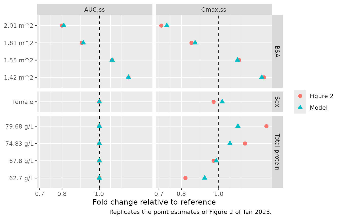

The AUC ratios follow directly from CL/F and match Figure 2 to within 0.01 for every level, and the BSA rows match for Cmax to within 0.03. The total-protein and sex rows for Cmax do not match; see Assumptions and deviations.

fig2_chk <- fig2 |> filter(covariate != "Reference")
stopifnot(
  # AUC: a closed-form consequence of the CL/F covariate model.
  all(abs(fig2_chk$auc_model - fig2_chk$auc_pub) < 0.02),
  # Cmax for BSA; a deterministic typical-value solve, so the bound only
  # needs to absorb the two-decimal rounding of the figure labels.
  all(abs(fig2_chk$cmax_model - fig2_chk$cmax_pub)[fig2_chk$covariate == "BSA"] < 0.04)
)

Single-dose profiles and NCA

The melanoma study opened with a single dose followed by sampling to 72 h (Table S1). The paper reports no NCA table of its own; it states that time to peak is within 3 h (Introduction; ‘ranging from 1 to 3 h’, Discussion) and that the terminal half-life is 31.8-57.4 h (Discussion). The simulation below follows single 4, 8 and 12 mg doses in a virtual melanoma cohort of 100 subjects per dose group, sampled to 14 days so the terminal phase is resolved.

rxode2::rxSetSeed(20230123)
set.seed(20230123)

# Covariates drawn to approximate Table S2 (FCN-159-001 column for melanoma,
# FCN-159-002 column for NF1). BSA is log-normal around the study median and
# total protein normal around it, each truncated to the reported range.
draw_covariates <- function(n, bsa_med, bsa_rng, tp_med, tp_rng, p_female, nf1) {
  tibble(
    BSA = pmin(pmax(exp(rnorm(n, log(bsa_med), 0.1)), bsa_rng[1]), bsa_rng[2]),
    TPRO = pmin(pmax(rnorm(n, tp_med, 5), tp_rng[1]), tp_rng[2]),
    SEXF = rbinom(n, 1, p_female),
    TUMTP_NF1 = nf1
  )
}

n_sd <- 100
sd_doses <- c(4, 8, 12)
sd_obs <- c(0, 0.25, 0.5, 0.75, 1, 1.25, 1.5, 2, 2.5, 3, 4, 6, 8, 12, 24, 48, 72,
            96, 120, 168, 240, 336)
sd_subjects <- bind_rows(lapply(seq_along(sd_doses), function(i) {
  draw_covariates(n_sd, 1.74, c(1.36, 2.16), 72.5, c(59, 82), 17 / 33, 0) |>
    mutate(id = (i - 1) * n_sd + seq_len(n_sd), dose = sd_doses[i])
}))
sd_events <- sd_subjects |>
  tidyr::crossing(tibble(time = c(0, sd_obs), evid = c(1, rep(0, length(sd_obs))))) |>
  mutate(
    amt = ifelse(evid == 1, dose, 0),
    cmt = ifelse(evid == 1, "depot", "central"),
    treatment = paste0(dose, " mg")
  ) |>
  arrange(id, time, desc(evid))
stopifnot(!anyDuplicated(unique(sd_events[, c("id", "time", "evid")])))

sd_sim <- rxode2::rxSolve(mod, events = sd_events, keep = c("treatment", "dose"),
                          returnType = "data.frame")
#> ℹ parameter labels from comments will be replaced by 'label()'

sd_sim |>
  filter(time > 0) |>
  group_by(treatment, time) |>
  summarise(
    Q05 = quantile(Cc, 0.05), Q50 = median(Cc), Q95 = quantile(Cc, 0.95),
    .groups = "drop"
  ) |>
  ggplot(aes(time, Q50)) +
  geom_ribbon(aes(ymin = Q05, ymax = Q95), alpha = 0.25) +
  geom_line() +
  facet_wrap(~treatment) +
  scale_y_log10() +
  labs(x = "Time after single dose (h)", y = "Luvometinib Cc (ng/mL)",
       caption = "Median and 90% prediction interval, melanoma patients.")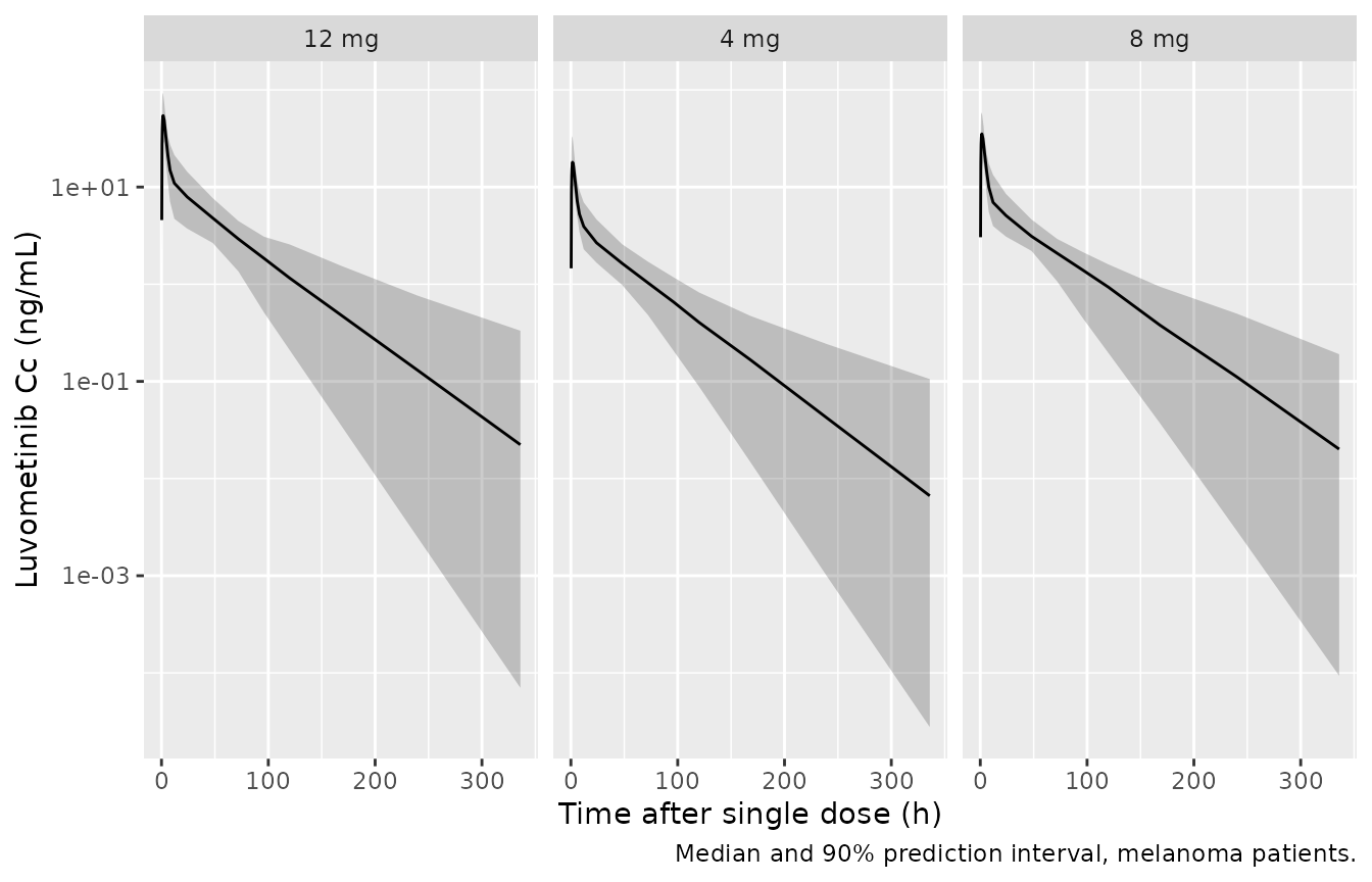

sd_conc <- sd_sim |>
  filter(!is.na(Cc)) |>
  select(id, time, Cc, treatment)
sd_conc <- bind_rows(
  sd_conc,
  sd_conc |> distinct(id, treatment) |> mutate(time = 0, Cc = 0)
) |>
  distinct(id, treatment, time, .keep_all = TRUE) |>
  arrange(id, treatment, time)

sd_dose <- sd_events |>
  filter(evid == 1) |>
  select(id, time, amt, treatment)

sd_nca <- PKNCA::pk.nca(PKNCA::PKNCAdata(
  PKNCA::PKNCAconc(sd_conc, Cc ~ time | treatment + id),
  PKNCA::PKNCAdose(sd_dose, amt ~ time | treatment + id),
  intervals = data.frame(start = 0, end = Inf, cmax = TRUE, tmax = TRUE,
                         aucinf.obs = TRUE, half.life = TRUE)
))

sd_summary <- as.data.frame(sd_nca) |>
  filter(PPTESTCD %in% c("cmax", "tmax", "aucinf.obs", "half.life")) |>
  group_by(treatment, PPTESTCD) |>
  summarise(median = median(PPORRES, na.rm = TRUE), .groups = "drop") |>
  pivot_wider(names_from = PPTESTCD, values_from = median)

sd_summary |>
  select(treatment, cmax, tmax, aucinf.obs, half.life) |>
  dplyr::rename(
    "Dose" = treatment, "Cmax (ng/mL)" = cmax, "Tmax (h)" = tmax,
    "AUC0-inf (ng*h/mL)" = aucinf.obs, "t1/2 (h)" = half.life
  ) |>
  knitr::kable(digits = 1, caption = "Median single-dose NCA of the simulated melanoma cohort.")

Median single-dose NCA of the simulated melanoma cohort.

Dose	Cmax (ng/mL)	Tmax (h)	AUC0-inf (ng*h/mL)	t1/2 (h)
12 mg	56.2	1.5	846.8	37.6
4 mg	18.9	1.5	292.6	34.9
8 mg	36.1	1.5	580.7	38.7

The median simulated Tmax is between 1 and 3 h as reported, and the median terminal half-life (about 35-39 h) lies inside the reported 31.8-57.4 h range. That range is not tied to a stated dose or population. In the model the half-life depends mainly on Vp/F, which is 75% larger in women, so women have the longer half-lives.

sd_hl <- as.data.frame(sd_nca) |> filter(PPTESTCD == "half.life")
sd_tmax <- as.data.frame(sd_nca) |> filter(PPTESTCD == "tmax")
stopifnot(
  # Tmax 'within 3 h' / 'from 1 to 3 h'; the typical-value Tmax is 1.7 h.
  median(sd_tmax$PPORRES) >= 1, median(sd_tmax$PPORRES) <= 3,
  # Half-life: the PKNCA cohort median is about 35-39 h per dose group. A
  # mis-transcribed peripheral volume or intercompartmental clearance moves it
  # by a factor of several.
  median(sd_hl$PPORRES, na.rm = TRUE) > 20,
  median(sd_hl$PPORRES, na.rm = TRUE) < 60
)

Pediatric BSA-band dosing (Figure 5)

The paper projected steady-state AUC0-24 in children aged 2-17 years by drawing BSA uniformly between 0.55 and 2.15 m^2 and assigning integer doses by BSA band, with between-subject variability and the adult bioavailability (Section 2.6). Figure 5 shows the resulting bands (2 mg for 0.55-0.7 m^2 up to 8 mg for 1.875-2.125 m^2, about 4 mg/m^2) alongside adults with NF1 at 8 mg. The box-plot medians below were digitised by the maintainers from the figure’s raster image (axis calibrated on its 0-2000 gridlines, about 3.3 ng*h/mL per pixel).

Children are simulated as NF1 patients; total protein is held at the 68.95 g/L reference and sex is drawn 50:50, neither of which affects AUC. The adult arm uses the pooled BSA distribution (the figure labels it 1.33-2.16 m^2) with NF1 bioavailability.

bands <- tibble::tribble(
  ~band,              ~lo,   ~hi,   ~dose, ~auc_fig5,
  "0.55-0.7 m^2",     0.55,  0.70,  2,     626,
  "0.71-0.85 m^2",    0.71,  0.85,  3,     714,
  "0.86-1.125 m^2",   0.86,  1.125, 4,     709,
  "1.126-1.375 m^2",  1.126, 1.375, 5,     668,
  "1.376-1.625 m^2",  1.376, 1.625, 6,     638,
  "1.626-1.875 m^2",  1.626, 1.875, 7,     615,
  "1.875-2.125 m^2",  1.875, 2.125, 8,     591
)
adult_fig5 <- 768

n_band <- 120
n_adult <- 200
ped_subjects <- bind_rows(lapply(seq_len(nrow(bands)), function(i) {
  tibble(
    id = (i - 1) * n_band + seq_len(n_band),
    BSA = runif(n_band, bands$lo[i], bands$hi[i]),
    TPRO = 68.95,
    SEXF = rbinom(n_band, 1, 0.5),
    TUMTP_NF1 = 1,
    dose = bands$dose[i],
    treatment = bands$band[i]
  )
}))
adult_subjects <- draw_covariates(n_adult, 1.66, c(1.33, 2.16), 71.75, c(59, 82), 19 / 45, 1) |>
  mutate(id = nrow(ped_subjects) + seq_len(n_adult), dose = 8, treatment = "Adults 8 mg")
fig5_subjects <- bind_rows(ped_subjects, adult_subjects)

ss_obs <- t_last + c(0, 0.25, 0.5, 0.75, 1, 1.25, 1.5, 2, 2.5, 3, 4, 6, 8, 12, 16, 20, 24)
fig5_events <- fig5_subjects |>
  tidyr::crossing(bind_rows(
    tibble(time = seq(0, t_last, by = tau), evid = 1),
    tibble(time = ss_obs, evid = 0)
  )) |>
  mutate(
    amt = ifelse(evid == 1, dose, 0),
    cmt = ifelse(evid == 1, "depot", "central")
  ) |>
  arrange(id, time, desc(evid))
stopifnot(!anyDuplicated(unique(fig5_events[, c("id", "time", "evid")])))

fig5_sim <- rxode2::rxSolve(mod, events = fig5_events, keep = c("treatment", "BSA"),
                            returnType = "data.frame")

fig5_conc <- fig5_sim |>
  filter(!is.na(Cc)) |>
  select(id, time, Cc, treatment)
fig5_dose <- fig5_events |>
  filter(evid == 1) |>
  select(id, time, amt, treatment)

fig5_nca <- PKNCA::pk.nca(PKNCA::PKNCAdata(
  PKNCA::PKNCAconc(fig5_conc, Cc ~ time | treatment + id),
  PKNCA::PKNCAdose(fig5_dose, amt ~ time | treatment + id),
  intervals = data.frame(start = t_last, end = t_last + tau, auclast = TRUE, cmax = TRUE)
))

fig5_published <- bind_rows(
  bands |> select(treatment = band, auclast = auc_fig5),
  tibble(treatment = "Adults 8 mg", auclast = adult_fig5)
)
fig5_cmp <- nlmixr2lib::ncaComparisonTable(
  simulated = fig5_nca,
  reference = fig5_published,
  by = "treatment",
  params = "auclast",
  units = c(auclast = "ng*h/mL"),
  tolerance_pct = 10
)
knitr::kable(
  fig5_cmp,
  caption = "Median steady-state AUC0-24: simulation vs Figure 5 of Tan 2023 (digitised). * differs by more than 10%."
)

Median steady-state AUC0-24: simulation vs Figure 5 of Tan 2023 (digitised). * differs by more than 10%.

NCA parameter	treatment	Reference	Simulated	% diff
AUClast (ng*h/mL)	0.55-0.7 m^2	626	595	-4.9%
AUClast (ng*h/mL)	0.71-0.85 m^2	714	650	-8.9%
AUClast (ng*h/mL)	0.86-1.125 m^2	709	689	-2.9%
AUClast (ng*h/mL)	1.126-1.375 m^2	668	675	+1.0%
AUClast (ng*h/mL)	1.376-1.625 m^2	638	673	+5.5%
AUClast (ng*h/mL)	1.626-1.875 m^2	615	661	+7.5%
AUClast (ng*h/mL)	1.875-2.125 m^2	591	625	+5.7%
AUClast (ng*h/mL)	Adults 8 mg	768	772	+0.6%

fig5_auc <- as.data.frame(fig5_nca) |>
  filter(PPTESTCD == "auclast") |>
  mutate(treatment = factor(treatment, levels = c(bands$band, "Adults 8 mg")))
ggplot(fig5_auc, aes(treatment, PPORRES, fill = treatment == "Adults 8 mg")) +
  geom_boxplot(outlier.shape = NA) +
  geom_point(data = fig5_published |>
               mutate(treatment = factor(treatment, levels = levels(fig5_auc$treatment))),
             aes(treatment, auclast), inherit.aes = FALSE, colour = "red", shape = 4, size = 3) +
  geom_hline(yintercept = adult_fig5, linetype = 2, colour = "red") +
  scale_fill_manual(values = c("white", "grey70"), guide = "none") +
  coord_cartesian(ylim = c(0, 2000)) +
  labs(x = NULL, y = "AUC0-24,ss (ng*h/mL)",
       caption = "Replicates Figure 5 of Tan 2023; red crosses are the digitised published medians.") +
  theme(axis.text.x = element_text(angle = 25, hjust = 1))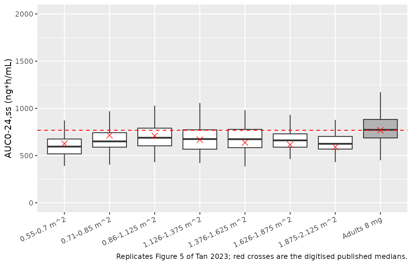

The simulated pediatric medians lie within about 10% of the published ones and the adult median within a few percent. The model’s pediatric medians fall more slowly with BSA than the published ones (higher in the largest bands, lower in the smallest); see Assumptions and deviations.

fig5_med <- fig5_auc |>
  group_by(treatment) |>
  summarise(median_auc = median(PPORRES), .groups = "drop") |>
  mutate(treatment = as.character(treatment)) |>
  inner_join(fig5_published, by = "treatment") |>
  mutate(pct_diff = 100 * (median_auc / auclast - 1))
stopifnot(
  nrow(fig5_med) == nrow(bands) + 1,
  # Typical-value AUCs differ from the digitised medians by -8% to +8%; the
  # simulated medians add about 2-3% sampling noise at 120 subjects per band
  # (one render gave -8.9% to +7.5%, median +1.0%). A mis-transcribed CL/F
  # or F1 shifts every band together and fails the median check.
  abs(median(fig5_med$pct_diff)) < 5,
  all(abs(fig5_med$pct_diff) < 15)
)

Assumptions and deviations

• Drug name. The paper uses the development code FCN-159; the file uses the INN luvometinib.
• IIV scale. Table 2 gives IIV as percentages without a formula. They are read as the coefficient of variation of a log-normal parameter and converted with omega^2 = log(1 + CV^2). Reading them as 100 x omega instead changes only Vc/F materially (variance 0.482 instead of 0.393). No covariance between etas was reported, so the etas are uncorrelated.
• Residual error. Methods 2.4.1 says combined additive and proportional error was used for model selection, but Results 3.2 and Table 2 report only a proportional term (25.8%), which is what the model uses.
• Total-protein reference. The Vc/F effect is centred on 68.95 g/L, the constant in the Table 1 equation and the forest-plot reference. Table S2 gives a pooled median of 71.75 g/L, so the centring value is not the tabulated median. The equation value is kept.
• Sex percentages. Table S2 prints the sex and diagnosis percentages against a denominator of 48 instead of 45 (26 men shown as 54.17%). The counts are used: 19 of 45 subjects (42.2%) were women.
• NF1 bioavailability. NF1 and melanoma patients came from separate studies, so the F1 effect is equally a study effect. The authors attribute it to bioavailability because both Cmax and AUC were higher in NF1.
• Figure 2, total protein and sex on Cmax (not reproduced). The model gives Cmax,ss ratios of 0.93, 0.99, 1.07 and 1.12 for total protein of 62.7, 67.8, 74.83 and 79.68 g/L, where Figure 2 shows 0.82, 0.97, 1.17 and 1.33. Results 3.3 likewise states a 30% higher Cmax,ss at 76.89 g/L, where the model gives about 9%. The published effect is about 2.6 times larger on the log scale than the printed exponent of -3.1 produces through Vc/F. The same model reproduces the BSA rows of the same figure, which also act through Vc/F (exponent 2.41), so the mismatch is specific to the total-protein term. No other reading of the Table 1 equation reproduces the figure, and parameters were not tuned to match it. Figure 2 also shows women with about 3% lower Cmax,ss than men, while the model gives about 2% higher, a difference of about 5 points from a 75% larger peripheral volume. Neither row is gated above.
• Figure 5 slope. The published pediatric medians fall from about 710 to 590 ng*h/mL between the 3 mg and 8 mg bands, which corresponds to a BSA exponent on CL/F near 1.24. The model, with the Table 2 exponent of 1.11, falls from about 680 to 640. The paper does not describe any change to the model for the pediatric simulation, so the Table 2 values are kept.
• Virtual cohorts. Covariate distributions are drawn to approximate Table S2: BSA log-normal (log-scale SD 0.1) around the study median and total protein normal (SD 5 g/L) around it, each truncated to the reported range. Children have BSA uniform within each band as in the paper, with total protein at the reference value; children are assumed to have the adult NF1 bioavailability, as in the paper.
• Figure 4 (VPC) pools several dose levels and two sampling schedules per panel without listing the per-subject doses, so it is not replicated.
• Errata. No correction notice is linked to the article in Europe PMC as of 2026-10-11.