Brexpiprazole with DM-3411 and DM-3412 metabolites (Frederiksen 2023)
Source:vignettes/articles/Frederiksen_2023_brexpiprazole.Rmd
Frederiksen_2023_brexpiprazole.RmdModel and source
- Citation: Frederiksen T, Areberg J, Raoufinia A, Schmidt E, Stage TB, Brosen K. Estimating the In Vivo Function of CYP2D6 Alleles through Population Pharmacokinetic Modeling of Brexpiprazole. Clin Pharmacol Ther. 2023 Feb;113(2):360-369. doi:10.1002/cpt.2791. PMCID: PMC10099095.
- Article: https://doi.org/10.1002/cpt.2791
The packaged model is the joint parent + two-metabolite population PK
model of Frederiksen 2023 (Figure 1b). Oral brexpiprazole is absorbed
first-order from a depot with a lag time into a
two-compartment disposition system (central +
peripheral1). The parent leaves central
only through two formation clearances, so its total
elimination clearance is their sum:
-
cl_form_dm3412(paperCL_M1) forms DM-3412, the minor metabolite, produced almost exclusively by CYP2D6. DM-3412 has two-compartment disposition (central_dm3412+peripheral1_dm3412). -
cl_form_dm3411(paperCL_M2) forms DM-3411, the major metabolite, produced mainly by CYP3A4 with a CYP2D6 contribution. DM-3411 has one-compartment disposition (central_dm3411).
Neither metabolite is believed to contribute to the pharmacological effect.
The point of the paper is the ratio between those two DM-3412 clearances. The Methods derive the DM-3412:brexpiprazole metabolic ratio (MR) as
because the fraction of parent clearance forming DM-3412 is , and the parent’s total clearance is that same denominator. The individual MR was then used as an in vivo surrogate of CYP2D6 activity in a genotype-phenotype regression. CYP2D6 genotype is not a covariate in the population PK model itself; it enters the paper only downstream. The two covariates that were retained are food state on the absorption rate constant and body-mass index on the DM-3411 central volume.
Population
pop <- readModelDb("Frederiksen_2023_brexpiprazole")()$population
str(pop, max.level = 1, give.attr = FALSE)
#> List of 16
#>  $ species       : chr "human"
#>  $ n_subjects    : num 826
#>  $ n_studies     : num 13
#>  $ age_range     : chr "18-65 years"
#>  $ age_median    : chr "36 years (IQR 27-46)"
#>  $ weight_range  : chr "32-159 kg"
#>  $ weight_median : chr "76 kg (IQR 65-90)"
#>  $ height_range  : chr "131-196 cm (median 170, IQR 164-177)"
#>  $ bmi_range     : chr "16-57 kg/m^2 (median 26, IQR 23-30)"
#>  $ sex_female_pct: num 35.7
#>  $ race_ethnicity: Named num [1:4] 61.1 17.9 19.5 1.5
#>  $ disease_state : chr "Pooled healthy subjects (179, 21.7%) and patients with schizophrenia (362, 43.8%), major depressive disorder (1"| __truncated__
#>  $ dose_range    : chr "Oral brexpiprazole 0.15-12 mg, single dose (phase I ascending-dose and PET studies) and multiple dose (multiple"| __truncated__
#>  $ regions       : chr "United States, Europe, Japan, Korea"
#>  $ genotype      : chr "CYP2D6 genotyped in all studies (TaqMan, DNA sequencing, and gel-based assays). CYP2D6 predicted phenotype in t"| __truncated__
#>  $ notes         : chr "Nine phase I and four phase II studies (Table S1). Plasma sampling was rich (>20 samples/subject, N = 245), sem"| __truncated__
The analysis pooled 13 clinical studies (9 phase I, 4 phase II) conducted in the United States, Europe, Japan, and Korea in 826 healthy subjects and patients with schizophrenia, major depressive disorder, or attention deficit hyperactivity disorder (Table 1 and Table S1). Oral doses spanned 0.15-12 mg as monotherapy (N = 541) or adjunctive treatment (N = 285). Plasma sampling was rich (> 20 samples/subject, N = 245), semi-sparse (8/subject, N = 314), or sparse (3-4/subject, N = 267), and the LC-MS/MS assay was linear over 0.300-100 ng/mL for all three analytes with an LLOQ of 0.300 ng/mL. Patients on moderate or strong CYP2D6 inhibitors were excluded and CYP3A4 inducers and inhibitors were disallowed throughout.
Baseline demographics of the population PK analysis set (Table 1): age median 36 years (IQR 27-46, range 18-65); weight median 76 kg (IQR 65-90, range 32-159); height median 170 cm; BMI median 26 kg/m^2 (IQR 23-30, range 16-57); 35.7% female; 61.1% White, 17.9% African American, 19.5% Asian, 1.5% Other.
Source trace
Every value in the packaged ini() block, with the
location it came from. Frederiksen 2023 reports the model in a single
table; the supplement’s Table S3 is a sensitivity analysis
(excluding subjects with no measurable DM-3412) and is
not the source of any packaged value.
| Parameter | Value | Source location |
|---|---|---|
| lka | 1.02 /h (fixed) | Table 2, ‘Absorption rate constant fasted’ |
| e_fed_ka | -0.47549 | Derived: Table 2 ka fed 0.535 / ka fasted 1.02 - 1 |
| ltlag | 0.411 h (fixed) | Table 2, ‘Lag-time’ |
| lvc | 81.2 L (fixed) | Table 2, ‘V2’ |
| lvp | 40.1 L (fixed) | Table 2, ‘V3’ |
| lq | 0.714 L/h (fixed) | Table 2, ‘Q’ |
| lcl_form_dm3412 | 0.0224 L/h | Table 2, ‘Clearance from brexpiprazole to DM-3412 (CLM1)’ |
| lcl_form_dm3411 | 1.12 L/h | Table 2, ‘Clearance from brexpiprazole to DM-3411 (CLM2)’ |
| lvc_dm3412 | 0.447 L | Table 2, ‘V4’ |
| lvp_dm3412 | 20.4 L | Table 2, ‘V5’ |
| lq_dm3412 | 2.16 L/h | Table 2, ‘QMET’ |
| lcl_dm3412 | 0.420 L/h | Table 2, ‘CLMET1’ |
| lvc_dm3411 | 2.44 L | Table 2, ‘V6’ |
| lcl_dm3411 | 3.33 L/h | Table 2, ‘CLMET2’ |
| e_bmi_vc_dm3411 | -0.0107 | Table 2, ‘Body mass index on V6’ (equation form not printed; see Errata) |
| etalka | 1.72678 (fixed) | Table 2 IIV 215% (fixed); log(2.15^2 + 1) |
| etalvc | 0.23688 | Table 2 IIV 51.7%; log(0.517^2 + 1) |
| etalvp | 0.44917 (fixed) | Table 2 IIV 75.3% (fixed); log(0.753^2 + 1) |
| etalcl_form_dm3412 | 0.52801 | Table 2 IIV 83.4%; log(0.834^2 + 1) |
| etalcl_form_dm3411 | 0.30396 | Table 2 IIV 59.6%; log(0.596^2 + 1) |
| etalvc_dm3412 | 1.70373 | Table 2 IIV 212%; log(2.12^2 + 1) |
| etalcl_dm3412 | 0.21916 | Table 2 IIV 49.5%; log(0.495^2 + 1) |
| etalvc_dm3411 | 0.95073 | Table 2 IIV 126%; log(1.26^2 + 1) |
| etalcl_dm3411 | 0.29259 | Table 2 IIV 58.3%; log(0.583^2 + 1) |
| propSd | 0.30610 | Table 2 ‘Residual error brexpiprazole’ 0.0937 (variance); sqrt() |
| propSd_dm3412 | 0.20543 | Table 2 ‘Residual error DM-3412’ 0.0422 (variance); sqrt() |
| propSd_dm3411 | 0.29120 | Table 2 ‘Residual error DM-3411’ 0.0848 (variance); sqrt() |
| ODE structure | 6 states | Figure 1b structural diagram + Results ‘Population pharmacokinetic analysis’ |
| MR = CLM1/CLMET1 | identity | Methods, ‘Estimating CYP2D6 activity’ |
The IIV conversion uses the Table 2 footnote,
%CV = sqrt(exp(omega^2) - 1) * 100, inverted to
omega^2 = log((CV/100)^2 + 1).
Typical-value simulation
A single oral 2 mg dose in the fasted state at the reference BMI of 26 kg/m^2. The 2 mg single dose matches the “AME, food effect” and DDI phase I studies of Table S1. Random effects are switched off, so this is the typical individual.
# rxode() turns the packaged model function into the rxUi object that carries
# $omega and $simulationModel; readModelDb() alone returns the function.
mod <- rxode2::rxode(readModelDb("Frederiksen_2023_brexpiprazole"))
mod_typ <- rxode2::zeroRe(mod, which = c("omega", "sigma"))

# Sampling grid: dense over the absorption and distribution phase, then coarse
# out to 1512 h. The parent's terminal half-life comes out at 91 h (see the NCA
# table below), so 1512 h is over 16 half-lives and AUC(0-1512) reaches
# AUC(0-inf) to within about 1e-5 of the total.
obs_times <- sort(unique(c(
  seq(0, 48, by = 0.25),
  seq(48, 1512, by = 6)
)))

# Route A event table (cmt = ODE state + explicit dvid). Built as a plain
# data.frame because rxode2::et() does not carry dvid through for multi-endpoint
# models.
make_events <- function(dose_mg, times, fed, bmi, id = 1L) {
  dosing <- data.frame(
    id = id, time = 0, amt = dose_mg, evid = 1L,
    cmt = "depot", dvid = NA_integer_
  )
  obs <- data.frame(
    id = id, time = times, amt = NA_real_, evid = 0L,
    cmt = "central", dvid = 1L
  )
  out <- dplyr::bind_rows(dosing, obs)
  out$FED <- fed
  out$BMI <- bmi
  dplyr::arrange(out, id, time, dplyr::desc(evid))
}

ev_typ <- make_events(dose_mg = 2, times = obs_times, fed = 0, bmi = 26)

# omega = NA is mandatory: rxode2 caches the previous solve's omega on the
# compiled model, so zeroRe() alone can silently leave IIV switched on.
typ <- rxode2::rxSolve(mod_typ, ev_typ, omega = NA)
typ <- as.data.frame(typ)
# A single-subject solve returns no `id` column; PKNCA needs one.
if (!"id" %in% names(typ)) typ$id <- 1L

# Guard that the typical-value solve really is typical.
stopifnot(dplyr::n_distinct(round(typ$cl_form_dm3412, 12)) == 1L)
stopifnot(dplyr::n_distinct(round(typ$vc_dm3411, 12)) == 1L)
prof <- typ |>
  dplyr::select(time, Brexpiprazole = Cc, `DM-3411` = Cc_dm3411, `DM-3412` = Cc_dm3412) |>
  tidyr::pivot_longer(-time, names_to = "Analyte", values_to = "conc") |>
  dplyr::filter(time <= 336)

ggplot(prof, aes(time, conc, colour = Analyte)) +
  geom_line(linewidth = 0.7) +
  scale_y_log10() +
  scale_x_continuous(breaks = seq(0, 336, by = 48)) +
  labs(x = "Time (h)", y = "Plasma concentration (ng/mL)",
       colour = NULL) +
  theme_bw()
#> Warning in scale_y_log10(): log-10 transformation introduced infinite values.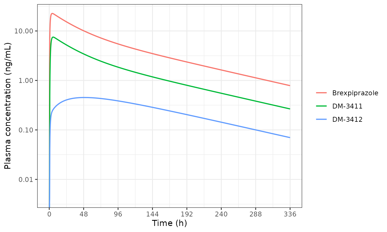
Typical-value plasma concentration-time profiles of brexpiprazole and its two metabolites after a single 2 mg oral dose, fasted, at BMI 26 kg/m^2. There is no published concentration-time figure to overlay: Frederiksen 2023 Figure 1 is the structural diagram, Figures 2-3 are per-subject metabolic-ratio boxplots, and the visual predictive check is supplementary Figure S2 (image only).
The profile shows the expected structure. Brexpiprazole declines with
a model-derived terminal half-life of about 91 h (see the NCA table
below); Frederiksen 2023 reports no half-life of its own, so this is a
property of the packaged parameters rather than a value to check against
the paper. DM-3411 equilibrates within a couple of hours
(cl_dm3411 / vc_dm3411 = 3.33 / 2.44 = 1.36 /h, a 0.5 h
half-life) and thereafter is formation-rate limited, tracking the parent
in parallel at about a third of its concentration. DM-3412 behaves the
same way at roughly a twentieth of the parent, and is close to the
paper’s 0.300 ng/mL LLOQ at this dose – consistent with the 160 of 826
subjects who had no DM-3412 measurement above the LLOQ.
PKNCA validation
There is no published NCA table in Frederiksen 2023 to compare against: the paper reports model parameters, not derived exposure metrics. Instead the NCA is used to test the model against the exact closed-form identities implied by the paper’s own Methods derivation, which is a much tighter gate than a percent-difference comparison against printed summary statistics.
For a linear system integrated to infinity, the mass entering each metabolite must equal the mass leaving it, giving
with the factor 1000 converting mg/L to ng/mL. The first of these is exactly the paper’s metabolic ratio.
nca_conc <- typ |>
  dplyr::select(id, time, Cc, Cc_dm3411, Cc_dm3412) |>
  tidyr::pivot_longer(c(Cc, Cc_dm3411, Cc_dm3412),
                      names_to = "analyte", values_to = "conc") |>
  dplyr::mutate(analyte = dplyr::recode(
    analyte, Cc = "Brexpiprazole", Cc_dm3411 = "DM-3411", Cc_dm3412 = "DM-3412"
  )) |>
  dplyr::filter(!is.na(conc))

nca_dose <- ev_typ |>
  dplyr::filter(evid == 1) |>
  dplyr::select(id, time, amt) |>
  tidyr::expand_grid(analyte = c("Brexpiprazole", "DM-3411", "DM-3412")) |>
  dplyr::select(id, time, amt, analyte)

conc_obj <- PKNCA::PKNCAconc(nca_conc, conc ~ time | analyte + id,
                             concu = "ng/mL", timeu = "h")
dose_obj <- PKNCA::PKNCAdose(nca_dose, amt ~ time | analyte + id,
                             doseu = "mg")

intervals <- data.frame(
  start     = 0,
  end       = max(obs_times),
  cmax      = TRUE,
  tmax      = TRUE,
  auclast   = TRUE,
  clast.obs = TRUE,
  half.life = TRUE
)

nca_res <- PKNCA::pk.nca(PKNCA::PKNCAdata(conc_obj, dose_obj, intervals = intervals))
nca_tab <- as.data.frame(nca_res)

nca_wide <- nca_tab |>
  dplyr::select(analyte, PPTESTCD, PPORRES) |>
  tidyr::pivot_wider(names_from = PPTESTCD, values_from = PPORRES)

nca_wide |>
  dplyr::select(analyte, cmax, tmax, auclast, half.life) |>
  dplyr::rename(
    "Analyte"            = analyte,
    "Cmax (ng/mL)"       = cmax,
    "Tmax (h)"           = tmax,
    "AUC0-1512 (ng*h/mL)" = auclast,
    "t1/2 (h)"           = half.life
  ) |>
knitr::kable(digits = c(0, 3, 2, 1, 1))| Analyte | Cmax (ng/mL) | Tmax (h) | AUC0-1512 (ng*h/mL) | t1/2 (h) |
|---|---|---|---|---|
| Brexpiprazole | 22.593 | 4.25 | 1750.9 | 91.2 |
| DM-3411 | 7.517 | 5.50 | 588.9 | 91.2 |
| DM-3412 | 0.452 | 48.00 | 93.4 | 92.1 |
p <- typ[1, ]

auc <- setNames(nca_wide$auclast, nca_wide$analyte)

# The paper's metabolic ratio, MR = CL_M1 / CL_MET1 (Methods).
mr_closed_form <- p$cl_form_dm3412 / p$cl_dm3412
mr_simulated   <- auc[["DM-3412"]] / auc[["Brexpiprazole"]]

# The DM-3411 analogue, CL_M2 / CL_MET2.
r3411_closed_form <- p$cl_form_dm3411 / p$cl_dm3411
r3411_simulated   <- auc[["DM-3411"]] / auc[["Brexpiprazole"]]

# The parent's own AUC: dose over total clearance (the sum of the two formation
# clearances, since the model gives the parent no other elimination route).
auc_closed_form <- 1000 * 2 / (p$cl_form_dm3412 + p$cl_form_dm3411)

identities <- tibble::tribble(
  ~Quantity, ~`Closed form`, ~Simulated,
  "MR = AUC(DM-3412) / AUC(brexpiprazole) = CL_M1 / CL_MET1",
    mr_closed_form, mr_simulated,
  "AUC(DM-3411) / AUC(brexpiprazole) = CL_M2 / CL_MET2",
    r3411_closed_form, r3411_simulated,
  "AUC(brexpiprazole) (ng*h/mL) = 1000 * dose / (CL_M1 + CL_M2)",
    auc_closed_form, auc[["Brexpiprazole"]]
) |>
  dplyr::mutate(`Relative difference (%)` =
                  100 * (Simulated - `Closed form`) / `Closed form`)

knitr::kable(identities, digits = c(0, 5, 5, 4))| Quantity | Closed form | Simulated | Relative difference (%) |
|---|---|---|---|
| MR = AUC(DM-3412) / AUC(brexpiprazole) = CL_M1 / CL_MET1 | 0.05333 | 0.05332 | -0.0236 |
| AUC(DM-3411) / AUC(brexpiprazole) = CL_M2 / CL_MET2 | 0.33634 | 0.33633 | -0.0029 |
| AUC(brexpiprazole) (ngh/mL) = 1000 dose / (CL_M1 + CL_M2) | 1750.70028 | 1750.88482 | 0.0105 |
# These are exact algebraic identities of the packaged ODE system, not
# statistical comparisons, so the tolerance is numerical (solver + trapezoidal
# AUC on a 6 h terminal grid), not biological.
stopifnot(
  abs(mr_simulated    / mr_closed_form    - 1) < 0.005,
  abs(r3411_simulated / r3411_closed_form - 1) < 0.005,
  abs(auc[["Brexpiprazole"]] / auc_closed_form - 1) < 0.005
)
The simulated metabolic ratio is 0.0533, reproducing the packaged
cl_form_dm3412 / cl_dm3412 = 0.0533. For context, the
paper’s observed per-subject median MRs were 0.088 for CYP2D6 normal
metabolizers, 0.045 for intermediate metabolizers, and 0.00074 for poor
metabolizers (Results, “CYP2D6 genotype-phenotype analysis”). The
typical-value MR sits between the intermediate- and normal-metabolizer
medians, which is what a population-typical value should do for a cohort
that was 44.7% normal metabolizers, 26.0% intermediate, and 2.8% poor.
The model carries no genotype covariate, so it cannot resolve the
phenotype strata itself – that separation lives entirely in the
between-subject variability on cl_form_dm3412.
Covariate checks
Food effect on the absorption rate constant
Food halves the absorption rate constant (1.02 -> 0.535 /h) and acts on nothing else, so it must delay and lower the parent peak while leaving total exposure exactly unchanged.
ev_fed <- make_events(dose_mg = 2, times = obs_times, fed = 1, bmi = 26)
fed <- as.data.frame(rxode2::rxSolve(mod_typ, ev_fed, omega = NA))

stopifnot(isTRUE(all.equal(fed$ka[1] / typ$ka[1], 0.535 / 1.02, tolerance = 1e-6)))

trapz <- function(x, y) sum(diff(x) * (utils::head(y, -1) + utils::tail(y, -1)) / 2)

food_tab <- tibble::tribble(
  ~State,   ~`ka (1/h)`,  ~`Cmax (ng/mL)`,      ~`Tmax (h)`,                  ~`AUC0-1512 (ng*h/mL)`,
  "Fasted", typ$ka[1],    max(typ$Cc),          typ$time[which.max(typ$Cc)],  trapz(typ$time, typ$Cc),
  "Fed",    fed$ka[1],    max(fed$Cc),          fed$time[which.max(fed$Cc)],  trapz(fed$time, fed$Cc)
)
knitr::kable(food_tab, digits = c(0, 3, 3, 2, 1))| State | ka (1/h) | Cmax (ng/mL) | Tmax (h) | AUC0-1512 (ng*h/mL) |
|---|---|---|---|---|
| Fasted | 1.020 | 22.593 | 4.25 | 1751.2 |
| Fed | 0.535 | 21.433 | 6.50 | 1751.2 |
Body-mass index on the DM-3411 central volume
BMI acts only on vc_dm3411. Because the
DM-3411 AUC is cl_form_dm3411 * AUC_parent / cl_dm3411, its
volume cancels out of the exposure entirely: BMI can change the DM-3411
peak and the speed of its early equilibration, but not its AUC. That is
a strong statement about how little this covariate does, and it is
consistent with the covariate’s marginal significance in the source
(19-point OFV drop, 95.3% RSE, upper 95% CI bound of -0.0000303).
bmi_levels <- c(16, 23, 26, 30, 57)  # Table 1 range, IQR bounds, and median
bmi_rows <- lapply(bmi_levels, function(b) {
  s <- as.data.frame(rxode2::rxSolve(
    mod_typ, make_events(2, obs_times, fed = 0, bmi = b), omega = NA
  ))
  data.frame(
    BMI = b,
    `V6 (L)` = s$vc_dm3411[1],
    `Cmax DM-3411 (ng/mL)` = max(s$Cc_dm3411),
    `AUC0-1512 DM-3411 (ng*h/mL)` = trapz(s$time, s$Cc_dm3411),
    check.names = FALSE
  )
})
bmi_tab <- dplyr::bind_rows(bmi_rows)
knitr::kable(bmi_tab, digits = c(0, 3, 3, 1))| BMI | V6 (L) | Cmax DM-3411 (ng/mL) | AUC0-1512 DM-3411 (ng*h/mL) |
|---|---|---|---|
| 16 | 2.701 | 7.496 | 589 |
| 23 | 2.518 | 7.511 | 589 |
| 26 | 2.440 | 7.517 | 589 |
| 30 | 2.336 | 7.524 | 589 |
| 57 | 1.631 | 7.567 | 589 |
Reproducing Table 3: the CYP2D6 activity scores
The paper’s headline result is Table 3, the CYP2D6 activity score (AS) for each allele. Those come from a multiple linear regression of log(MR) on per-allele indicator counts, not from the ODE model, but reproducing them confirms that the metabolic ratio has been read correctly. The Methods state that CYP2D6*1 is fixed to AS 1, the pooled null alleles to AS 0, and that every other allele’s AS is “the relative activity to CYP2D6*1 adjusted by the contribution from the null function alleles”. The equation printed there is the linear rescaling that sends the null estimate to 0 and the *1 estimate to 1,
applied to the exponentially back-transformed regression coefficients in the “CYP2D6 activity estimate” column of Table 3.
tab3 <- tibble::tribble(
  ~Allele,        ~n,  ~`Activity estimate`, ~`AS published`,
  "CYP2D6*null",  176, 0.24, 0.00,
  "CYP2D6*1",     396, 0.92, 1.00,
  "CYP2D6*2",     183, 0.31, 0.10,
  "CYP2D6*9",      20, 0.40, 0.23,
  "CYP2D6*10",     62, 0.46, 0.32,
  "CYP2D6*14",      1, 0.68, 0.64,
  "CYP2D6*17",     37, 0.27, 0.04,
  "CYP2D6*29",     13, 0.27, 0.04,
  "CYP2D6*41",     64, 0.30, 0.09
)

b_null <- tab3$`Activity estimate`[tab3$Allele == "CYP2D6*null"]
b_wt   <- tab3$`Activity estimate`[tab3$Allele == "CYP2D6*1"]

tab3 <- tab3 |>
  dplyr::mutate(
    `AS recomputed` = round((`Activity estimate` - b_null) / (b_wt - b_null), 2),
    # Work in integer hundredths so the comparison below is exact rather than
    # tripping over 0.24 - 0.23 == 0.010000000000000009 in binary floating point.
    Difference      = round(100 * (`AS recomputed` - `AS published`))
  )

tab3 |>
  dplyr::rename(
    "Number of alleles"          = n,
    "Difference (0.01 units)"    = Difference
  ) |>
knitr::kable(digits = c(0, 0, 2, 2, 2, 0))| Allele | Number of alleles | Activity estimate | AS published | AS recomputed | Difference (0.01 units) |
|---|---|---|---|---|---|
| CYP2D6*null | 176 | 0.24 | 0.00 | 0.00 | 0 |
| CYP2D6*1 | 396 | 0.92 | 1.00 | 1.00 | 0 |
| CYP2D6*2 | 183 | 0.31 | 0.10 | 0.10 | 0 |
| CYP2D6*9 | 20 | 0.40 | 0.23 | 0.24 | 1 |
| CYP2D6*10 | 62 | 0.46 | 0.32 | 0.32 | 0 |
| CYP2D6*14 | 1 | 0.68 | 0.64 | 0.65 | 1 |
| CYP2D6*17 | 37 | 0.27 | 0.04 | 0.04 | 0 |
| CYP2D6*29 | 13 | 0.27 | 0.04 | 0.04 | 0 |
| CYP2D6*41 | 64 | 0.30 | 0.09 | 0.09 | 0 |
# Table 3 prints the regression estimates to only two decimal places, so the
# recomputation inherits a rounding granularity of about +/- 0.01 on the
# rescaled score. Seven of the nine rows land exactly; *9 and *14 are one unit
# in the last place high. A wrong formula would not land within 0.01 on all
# nine rows, so this is the rounding floor and not a structural mismatch.
stopifnot(
  max(abs(tab3$Difference)) <= 1L,
  sum(tab3$Difference == 0L) >= 7L
)
Seven of the nine rows reproduce the published activity score exactly and the remaining two (*9 and *14) are high by 0.01, which is the rounding floor imposed by Table 3 printing its regression estimates to two decimal places. That the formula lands within one unit in the last place on every allele – including the two anchors it is constructed to fix, *null at 0.00 and *1 at 1.00 – confirms the transcription of Table 3 against the Methods equation. The result the paper draws from it is that CYP2D6*2 – conventionally a fully functional allele – carries only 10% of wild-type activity toward brexpiprazole, and that the decreased-function alleles *17, *29, and *41 sit at 4-9% rather than the 0.5 an activity-score system would assign them.
Population simulation
A 200-subject cohort at 4 mg once daily for 28 days, with BMI drawn to match the Table 1 distribution (median 26, IQR 23-30 kg/m^2), fasted dosing.
set.seed(20230201)
rxode2::rxSetSeed(20230201)

n_sub <- 200
tau <- 24
n_days <- 28

# Log-normal BMI matched to the Table 1 median and IQR, truncated to the
# observed 16-57 kg/m^2 range.
bmi_sd <- log(30 / 23) / (2 * qnorm(0.75))
subj <- data.frame(
  id = seq_len(n_sub),
  BMI = pmin(57, pmax(16, exp(rnorm(n_sub, log(26), bmi_sd))))
)

ss_times <- sort(unique(c(
  seq(0, n_days * tau, by = 6),
  (n_days - 1) * tau + seq(0, tau, by = 0.5)
)))

pop_dose <- tidyr::expand_grid(
  id = subj$id, time = seq(0, (n_days - 1) * tau, by = tau)
) |>
  dplyr::mutate(amt = 4, evid = 1L, cmt = "depot", dvid = NA_integer_)

pop_obs <- tidyr::expand_grid(id = subj$id, time = ss_times) |>
  dplyr::mutate(amt = NA_real_, evid = 0L, cmt = "central", dvid = 1L)

ev_pop <- dplyr::bind_rows(pop_dose, pop_obs) |>
  dplyr::left_join(subj, by = "id") |>
  dplyr::mutate(FED = 0) |>
  dplyr::arrange(id, time, dplyr::desc(evid))

# omega must be passed explicitly: an earlier zeroRe() solve in this session
# otherwise leaves the compiled model's cached omega switched off, silently
# collapsing all 200 subjects onto the typical individual.
pop <- as.data.frame(rxode2::rxSolve(
  mod$simulationModel, ev_pop, omega = mod$omega,
  keep = c("BMI", "FED")
))

# Guard that IIV really is switched on.
stopifnot(dplyr::n_distinct(round(pop$cl_form_dm3412, 8)) > 1L)

# Cc is the individual prediction and `sim` is the one carrying residual error.
# The pre-lag rows have Cc exactly 0, where a proportional-only error model
# leaves ipredSim/sim as NA, so the comparison is made on the informative rows.
err_rows <- !is.na(pop$ipredSim)
stopifnot(
  any(err_rows),
  isTRUE(all.equal(pop$Cc[err_rows], pop$ipredSim[err_rows])),
  !isTRUE(all.equal(pop$Cc[err_rows], pop$sim[err_rows]))
)
# The figures below use Cc (the individual prediction), not `sim`: assay noise
# would blur the percentile ribbons without making them more faithful to the
# published model.
ss <- pop |>
  dplyr::filter(time >= (n_days - 1) * tau) |>
  dplyr::mutate(tad = time - (n_days - 1) * tau) |>
  dplyr::select(id, tad, Brexpiprazole = Cc, `DM-3411` = Cc_dm3411, `DM-3412` = Cc_dm3412) |>
  tidyr::pivot_longer(-c(id, tad), names_to = "Analyte", values_to = "conc") |>
  dplyr::group_by(Analyte, tad) |>
  dplyr::summarise(
    p05 = quantile(conc, 0.05), p50 = median(conc), p95 = quantile(conc, 0.95),
    .groups = "drop"
  )

ggplot(ss, aes(tad, p50, colour = Analyte, fill = Analyte)) +
  geom_ribbon(aes(ymin = p05, ymax = p95), alpha = 0.18, colour = NA) +
  geom_line(linewidth = 0.7) +
  scale_y_log10() +
  scale_x_continuous(breaks = seq(0, 24, by = 4)) +
  labs(x = "Time after dose (h)", y = "Plasma concentration (ng/mL)",
       colour = NULL, fill = NULL) +
  theme_bw()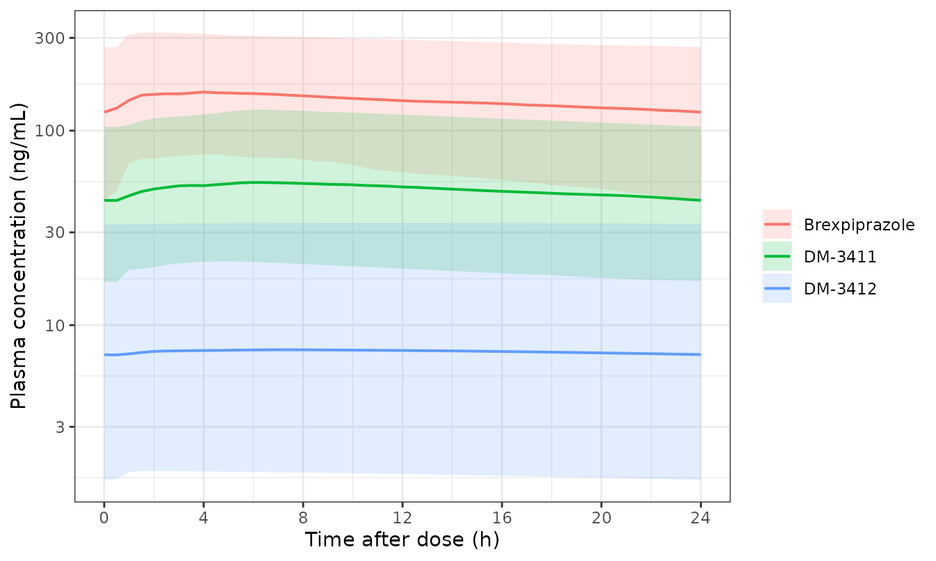
Simulated steady-state profiles over the final 24 h dosing interval of 4 mg once-daily brexpiprazole in 200 subjects: median and 5th-95th percentiles for the parent and both metabolites. Compare with the layout of supplementary Figure S2 (visual predictive check), which the source provides as an image only.
# Per-subject metabolic ratio from the individual parameters, exactly as the
# paper computed it from the empirical Bayes estimates.
mr_pop <- pop |>
  dplyr::group_by(id) |>
  dplyr::summarise(MR = dplyr::first(cl_form_dm3412) / dplyr::first(cl_dm3412),
                   .groups = "drop")

mr_summary <- tibble::tibble(
  Statistic = c("Median", "5th percentile", "95th percentile",
                "Geometric SD of MR", "Typical value (CL_M1 / CL_MET1)"),
  Value = c(median(mr_pop$MR), quantile(mr_pop$MR, 0.05),
            quantile(mr_pop$MR, 0.95), exp(sd(log(mr_pop$MR))),
            mr_closed_form)
)
knitr::kable(mr_summary, digits = 4)| Statistic | Value |
|---|---|
| Median | 0.0484 |
| 5th percentile | 0.0129 |
| 95th percentile | 0.2130 |
| Geometric SD of MR | 2.3796 |
| Typical value (CL_M1 / CL_MET1) | 0.0533 |
# The MR is a ratio of two independent log-normals, so its population median
# must equal the typical value. Assert on the centre, never on the extremes of
# a random cohort.
stopifnot(abs(median(mr_pop$MR) / mr_closed_form - 1) < 0.20)

# The model's total between-subject spread in log(MR) is the sum of the two
# component IIV variances, since the ini() block has a diagonal Omega.
sd_log_mr_expected <- sqrt(0.52801 + 0.21916)
stopifnot(abs(sd(log(mr_pop$MR)) / sd_log_mr_expected - 1) < 0.20)
The simulated MR distribution spans roughly the range the paper’s Figure 2 covers across genotypes. Its total between-subject SD on the log scale is 0.864, since the packaged Omega is diagonal and the MR is the ratio of two log-normal parameters. The paper reports that CYP2D6 alleles explained 67% of the variability in MR (adjusted R^2 = 0.67), so about a third of this simulated spread corresponds to the within-genotype residual the paper attributes to unmeasured enzyme-expression and environmental factors. Because the packaged model carries no genotype covariate, the simulated distribution is unstratified: it cannot be read as a phenotype prediction.
Assumptions and deviations (Errata)
Residual-error scale is an interpretation, not a printed fact. Table 2 labels the three residual-error rows only as “Residual error brexpiprazole / DM-3412 / DM-3411” with bare values 0.0937, 0.0422, and 0.0848 and no scale. They are read here as NONMEM
$SIGMAvariances, so the packaged proportional SDs are their square roots (30.6%, 20.5%, and 29.1%). Two reasons: the paper explicitly converts the OMEGA values to %CV under a table footnote but attaches no such footnote to the SIGMA rows, i.e. it leaves them on the native NONMEM scale; and 20-31% residual CVs are the expected magnitude for pooled rich-plus-sparse phase I/II data, whereas reading the values as SDs would imply an implausible 4-9% residual CV across three analytes including one that is frequently below the LLOQ.The three IIV covariance blocks are not reproduced. The Results state that the final model included covariances among V2-CLM1-CLM2, V4-CLMET1, and V6-CLMET2, but no covariance, correlation, or off-diagonal value is reported anywhere – not in the text, not in Table 2, and not in the Supplementary Material (Tables S1-S3 were checked). The packaged Omega is therefore diagonal. Simulated cohorts will show no between-subject correlation among those parameter pairs, and the marginal variances are correct while the joint distribution is not.
The BMI-on-V6 equation form and centring value are not printed. Table 2 gives the coefficient -0.0107 but the paper never writes the covariate equation. The packaged model uses the linear-deviation form
vc_dm3411 * (1 + e_bmi_vc_dm3411 * (BMI - 26)), which is the form documented forBMIininst/references/covariate-columns.md, with the reference 26 kg/m^2 taken as the population PK analysis set’s median BMI (Table 1). A power form(BMI/26)^-0.0107is excluded because it would move V6 by under 1% across the entire 16-57 kg/m^2 observed range and so could not have produced the reported 19-point OFV drop. An exponential formexp(-0.0107 * (BMI - 26))is numerically indistinguishable from the linear form across the interquartile range (both within 0.1%) and differs by 7% only at the extreme BMI of 57. As shown above, this covariate does not affect DM-3411 exposure at all under either form.e_fed_kais a re-parameterisation, not a printed coefficient. Table 2 reports two absorption rate constants rather than a fractional effect. The packagede_fed_ka = 0.535 / 1.02 - 1 = -0.47549reproduces both printed values exactly and matches the canonicalFEDlinear-deviation convention. The Discussion cautions that the food effect “appeared to be driven by individuals from a multiple-ascending dose study” and that a dedicated food-effect study found no impact on brexpiprazole PK, so this coefficient is better read as a study-confounded absorption-rate difference than as an established prandial effect.All clearances and volumes are apparent (CL/F, V/F). Every pooled study dosed orally and no absolute bioavailability was estimated, so
lfdepotis absent by construction rather than fixed to 1.The metabolite states carry brexpiprazole-mass equivalents. The formation clearances are apparent, so the DM-3411 / DM-3412 molar-mass ratios and metabolite bioavailabilities are absorbed into V4, V5, and V6, exactly as in the NONMEM fit. This is why V4 = 0.447 L is a physically implausible volume read literally; it is not one.
The Table 2 bootstrap confidence intervals for the DM-3412 parameters do not contain their point estimates, which the paper states outright (“the parameters related to DM-3412 (CLM1, V4, V5, CLMET1, and QMET) were all outside the 95% confidence intervals”). It attributes this to the below-LLOQ DM-3412 observations and shows in Table S3 that excluding subjects with no measurable DM-3412 restores the precision. The packaged model uses the final model’s point estimates (Table 2), not the Table S3 sensitivity estimates. Note also that the supplement’s Table S3 reprints Table 2’s confidence-interval column verbatim while showing different point estimates, and prints its IIV column as variances rather than as the %CV Table 2 uses; neither table S3 quirk affects the packaged values.
No published NCA comparison is possible. Frederiksen 2023 reports no Cmax, Tmax, AUC, or half-life values for any analyte. The PKNCA section above therefore validates against the exact closed-form identities implied by the paper’s own Methods derivation of the metabolic ratio, which is a stricter test than a tolerance comparison against printed summary statistics would be.
CYP2D6 genotype is deliberately absent from the model. It is the paper’s subject but not a covariate in the population PK model; it enters only through the downstream metabolic-ratio regression reproduced above. A user who wants genotype-specific exposure must apply the Table 3 activity scores to
cl_form_dm3412themselves, and should note that the paper does not publish the mapping from activity score to a CLM1 multiplier.The virtual cohort’s BMI distribution is assumed log-normal. Table 1 reports only the median and interquartile range, so the log-normal parameters were back-solved from those and truncated to the reported 16-57 kg/m^2 range. This affects only the population figure, not any of the identity checks.