Fosmidomycin + clindamycin with artesunate for falciparum malaria (Pfaffendorf 2026)
Source:vignettes/articles/Pfaffendorf_2026_fosmidomycin_clindamycin.Rmd
Pfaffendorf_2026_fosmidomycin_clindamycin.RmdModel and source
Pfaffendorf 2026 fitted fosmidomycin and clindamycin separately (“Each compound was modeled separately”, Methods / Structural model selection), so the paper contributes two independent model files that share this one vignette.
fosUi <- rxode2::rxode(readModelDb("Pfaffendorf_2026_fosmidomycin"))
#> ℹ parameter labels from comments will be replaced by 'label()'
cliUi <- rxode2::rxode(readModelDb("Pfaffendorf_2026_clindamycin"))
#> ℹ parameter labels from comments will be replaced by 'label()'
#> Warning: some etas defaulted to non-mu referenced, possible parsing error: etaiov_cl_1, etaiov_cl_2, etaiov_cl_3, etaiov_cl_4, etaiov_cl_5, etaiov_cl_6
#> as a work-around try putting the mu-referenced expression on a simple line- Citation: Pfaffendorf C, Dejon-Agobe JC, Edoa JR, Maiga-Ascofare O, Ahenkan E, Adegnika AA, Ramharter M, Wicha SG, Mischlinger J (2026). Population pharmacokinetics of fosmidomycin and clindamycin in combination with artesunate for uncomplicated Plasmodium falciparum malaria in Gabonese children and adults. Malaria Journal 25:152. doi:10.1186/s12936-026-05872-6. Parameter values from Table 2 (fosmidomycin block); model structure from Additional file 1 section S2 (final NONMEM control stream).
- Fosmidomycin: Population PK model for oral fosmidomycin co-administered with clindamycin and artesunate in Gabonese children and adults with uncomplicated Plasmodium falciparum malaria (Pfaffendorf 2026). One-compartment disposition with linear elimination, first-order absorption and an absorption lag time. Allometric body-weight scaling is applied with fixed exponents 0.75 on apparent clearance and 1 on apparent volume, centered at the cohort median weight of 29.05 kg. Body temperature increases apparent clearance as a power function centered at the cohort mean 37.1 degC. Relative bioavailability is fixed at 1 and carries log-normal IIV; further IIV is carried on the absorption rate constant. Residual error is combined proportional plus additive.
- Clindamycin: Population PK model for oral clindamycin co-administered with fosmidomycin and artesunate in Gabonese children and adults with uncomplicated Plasmodium falciparum malaria (Pfaffendorf 2026). One-compartment disposition with linear elimination, first-order absorption and an absorption lag time. Allometric body-weight scaling is applied with fixed exponents 0.75 on apparent clearance and 1 on apparent volume, centered at the cohort median weight of 29.05 kg; no other covariate was retained. Correlated log-normal IIV is carried on the absorption rate constant and the lag time, and inter-occasion variability on apparent clearance across the six dosing occasions. Residual error is combined proportional plus additive.
- Article: https://doi.org/10.1186/s12936-026-05872-6
- Supplement (Additional file 1, DOCX): contains the demographic listing (S1), the final NONMEM control streams for fosmidomycin (S2) and clindamycin (S3), goodness-of-fit plots (S4, S5), the pairwise exposure tests (S6, S7) and the proposed clindamycin weight-band dosing table (S8).
Both models are one-compartment with first-order absorption and an
absorption lag time (NONMEM ADVAN2 TRANS2), with allometric
body-weight scaling at fixed exponents 0.75 on CL/F and 1 on V/F centred
at 29.05 kg. Fosmidomycin additionally carries a power effect of body
temperature on CL/F.
Population
Forty patients aged 3.5 to 57.2 years (median 10.8) with microscopically confirmed uncomplicated Plasmodium falciparum mono-infection were enrolled at the Centre de Recherches Medicales de Lambarene, Gabon, within an open-label randomised phase II trial (PACTR202008909968293). Recruitment was stratified into three age strata: 20 children aged 6 months to 10 years, 10 adolescents aged 11 to 17 years, and 10 adults aged 18 to 65 years. Baseline characteristics (Table 1): weight mean (SD) 37.5 (20.2) kg, median [min, max] 29.1 [12.0, 86.0] kg; body temperature 37.1 (1.06) degC, median [min, max] 36.8 [35.4, 39.0] degC; GFR 126 (34.9) mL/min/1.73m2; haemoglobin 10.9 (1.39) g/dL; albumin 36.0 (5.49) g/L; 17/40 (42.5%) female.
All patients received oral artesunate 2 mg/kg, fosmidomycin 30 mg/kg and clindamycin 10 mg/kg every 12 h for three days (six doses). 242 fosmidomycin and 274 clindamycin plasma concentrations entered the analysis, assayed by LC-MS/MS over calibration ranges of 0.25-15 mg/L and 0.005-0.5 mg/L respectively, with below-quantification data handled by the M3 method.
The same information is available programmatically via each model’s
population metadata,
e.g. fosUi$population.
Source trace
Every ini() entry carries an in-file comment naming its
origin. Table 2 of the paper and the $THETA /
$OMEGA / $SIGMA records of the final control
streams in Additional file 1 (S2, S3) agree on every value, which
confirms these are final estimates rather than initial
values.
| Equation / parameter | Value | Source location |
|---|---|---|
| Fosmidomycin | ||
lcl (CL/F at 29.05 kg, 37.1 degC) |
58.3 L/h | Table 2; S2 $THETA (0, 58.3) ;1_CL
|
lvc (V/F at 29.05 kg) |
248 L | Table 2; S2 $THETA (0, 248) ;2_V
|
lka |
0.698 1/h | Table 2; S2 $THETA (0, 0.698) ;3_KA
|
ltlag |
0.105 h | Table 2; S2 $THETA (0, 0.105) ;4_ALAG1
|
lfdepot |
1 FIXED | Table 2; S2 $THETA (1) FIX ;5_F1
|
e_wt_cl, e_wt_vc
|
0.75, 1 (fixed) | Methods “Covariate model building”; S2 $PK
|
e_bodytemp_cl |
6.68 | Table 2 theta_TEMP; S2
$THETA (-100, 6.68, 100000) ;6_CLBT1
|
etalka |
0.383 (68.3% CV) | S2 $OMEGA 0.383 ;2_IIV_KA; Table 2 omega_ka |
etalfdepot |
0.114 (34.7% CV) | S2 $OMEGA 0.114 ;3_IIV_F1; Table 2 omega_F |
propSd, addSd
|
0.3564, 0.1972 mg/L | S2 $SIGMA 0.127 / 0.0389; Table 2 sigma rows |
d/dt(depot), d/dt(central),
f(depot), alag(depot)
|
n/a | S2 $SUBROUTINES ADVAN2 TRANS2, $PK
|
CL_i = CL_TV*(WGT/29.05)^0.75*(BT/37.1)^theta_TEMP |
n/a | Results “Fosmidomycin model”, unnumbered equation; S2
$PK TVCL
|
V_i = V_TV*(WGT/29.05)^1 |
n/a | Results “Fosmidomycin model”, unnumbered equation; S2
$PK TVV
|
| Clindamycin | ||
lcl (CL/F at 29.05 kg) |
8.02 L/h | Table 2; S3 $THETA (0.001, 8.02) ;1_CL
|
lvc (V/F at 29.05 kg) |
28.4 L | Table 2; S3 $THETA (0.001, 28.4) ;2_Vc
|
lka |
2.2 1/h | Table 2; S3 $THETA (0.001, 2.2) ;3_KA
|
ltlag |
0.227 h | Table 2; S3 $THETA (0, 0.227) ;5_LAG-Time
|
lfdepot |
1 FIXED | S3 $THETA (1) FIX ;4_F1 (no Table 2 row) |
e_wt_cl, e_wt_vc
|
0.75, 1 (fixed) | Methods “Covariate model building”; S3 $PK
|
etalka + etaltlag block |
0.611 / -0.0524 / 0.0114 | S3 $OMEGA BLOCK(2); Table 2 omega_ka 91.8%, omega_tlag
10.7%, corr -63% |
etaiov_cl_1 .. _6
|
0.0798 (28.8% CV) | S3 $OMEGA BLOCK(1) 0.0798 + 5 SAME; Table
2 kappa_CL/F |
propSd, addSd
|
0.3286, 0.004111 mg/L | S3 $SIGMA 0.108 / 1.69E-05; Table 2 sigma rows |
CL_i = CL_TV*(WGT/29.05)^0.75 |
n/a | Results “Clindamycin model”, unnumbered equation; S3
$PK TVCL
|
Residual model
Y = IPRED + IPRED*eps_prop + eps_add
|
n/a | Methods “Residual variability model”; S2 / S3
$ERROR
|
The Table 2 %CV columns are reproduced from the control-stream
variances by CV = sqrt(exp(omega^2) - 1) * 100, and the
reported ka / lag correlation by
cov / sqrt(var_ka * var_tlag):
cvpct <- function(v) sqrt(exp(v) - 1) * 100
scaleChk <- tibble::tribble(
  ~Quantity,                        ~`Control stream`, ~Derived,             ~`Table 2`,
  "fosmidomycin omega_ka (%CV)",     0.383,            cvpct(0.383),          68.3,
  "fosmidomycin omega_F (%CV)",      0.114,            cvpct(0.114),          34.7,
  "fosmidomycin sigma_prop (%CV)",   0.127,            sqrt(0.127) * 100,     35.6,
  "fosmidomycin sigma_add (mg/L)",   0.0389,           sqrt(0.0389),           0.197,
  "clindamycin omega_ka (%CV)",      0.611,            cvpct(0.611),          91.8,
  "clindamycin omega_tlag (%CV)",    0.0114,           cvpct(0.0114),         10.7,
  "clindamycin ka/tlag corr (%)",   -0.0524,          -0.0524 / sqrt(0.611 * 0.0114) * 100, -63,
  "clindamycin kappa_CL (%CV)",      0.0798,           cvpct(0.0798),         28.8,
  "clindamycin sigma_prop (%CV)",    0.108,            sqrt(0.108) * 100,     32.9,
  "clindamycin sigma_add (mg/L)",    1.69e-05,         sqrt(1.69e-05),         0.0041
)
# Every derived value must land on the printed Table 2 value to within the
# rounding of the printed column. This pins the OMEGA / SIGMA scale: if the
# variances were actually SDs (or CVs), these would disagree by large factors.
stopifnot(
  with(scaleChk, all(abs(Derived - `Table 2`) <= 0.05 * pmax(abs(`Table 2`), 1e-4)))
)
knitr::kable(scaleChk, digits = 5,
caption = "Control-stream variances reproduce the Table 2 %CV / SD columns.")| Quantity | Control stream | Derived | Table 2 |
|---|---|---|---|
| fosmidomycin omega_ka (%CV) | 0.38300 | 68.31384 | 68.3000 |
| fosmidomycin omega_F (%CV) | 0.11400 | 34.74941 | 34.7000 |
| fosmidomycin sigma_prop (%CV) | 0.12700 | 35.63706 | 35.6000 |
| fosmidomycin sigma_add (mg/L) | 0.03890 | 0.19723 | 0.1970 |
| clindamycin omega_ka (%CV) | 0.61100 | 91.77542 | 91.8000 |
| clindamycin omega_tlag (%CV) | 0.01140 | 10.70758 | 10.7000 |
| clindamycin ka/tlag corr (%) | -0.05240 | -62.78534 | -63.0000 |
| clindamycin kappa_CL (%CV) | 0.07980 | 28.82194 | 28.8000 |
| clindamycin sigma_prop (%CV) | 0.10800 | 32.86335 | 32.9000 |
| clindamycin sigma_add (mg/L) | 0.00002 | 0.00411 | 0.0041 |
Deterministic checks against the paper’s own numbers
These use zeroRe() so they are exact typical-value
quantities with no cohort draw: the tolerances can therefore be tight
and are not subject to the thread-count cohort variation that affects
the stochastic sections below.
WTREF <- 29.05    # Methods, VPC: median weight of the study population
BTREF <- 37.1     # Methods, VPC: reference body temperature

doseGrid <- sort(unique(c(seq(0, 96, by = 0.25),
                          as.vector(outer(seq(0, 60, by = 12), seq(0, 6, by = 0.05), "+")))))
doseGrid <- doseGrid[doseGrid <= 96]

# --- fosmidomycin, single 900 mg dose at the VPC reference subject ---------
evFos <- rxode2::et(amt = 900, cmt = "depot") |>
  rxode2::et(doseGrid, cmt = "central") |>
  as.data.frame() |>
  dplyr::mutate(WT = WTREF, BODYTEMP = BTREF)
sFos <- rxode2::rxSolve(rxode2::zeroRe(fosUi), evFos, returnType = "data.frame")
#> ℹ omega/sigma items treated as zero: 'etalka', 'etalfdepot'

# --- clindamycin, single 290.5 mg (10 mg/kg) dose --------------------------
evCli <- rxode2::et(amt = 10 * WTREF, cmt = "depot") |>
  rxode2::et(doseGrid, cmt = "central") |>
  as.data.frame() |>
  dplyr::mutate(WT = WTREF, OCC = 1)
sCli <- rxode2::rxSolve(rxode2::zeroRe(cliUi), evCli, returnType = "data.frame")
#> Warning: some etas defaulted to non-mu referenced, possible parsing error: etaiov_cl_1, etaiov_cl_2, etaiov_cl_3, etaiov_cl_4, etaiov_cl_5, etaiov_cl_6
#> as a work-around try putting the mu-referenced expression on a simple line
#> ℹ omega/sigma items treated as zero: 'etalka', 'etaltlag', 'etaiov_cl_1', 'etaiov_cl_2', 'etaiov_cl_3', 'etaiov_cl_4', 'etaiov_cl_5', 'etaiov_cl_6'

hlFos <- PKNCA::pk.calc.half.life(conc = sFos$Cc, time = sFos$time)$half.life
hlCli <- PKNCA::pk.calc.half.life(conc = sCli$Cc, time = sCli$time)$half.life
aucFos <- PKNCA::pk.calc.auc.last(conc = sFos$Cc, time = sFos$time)
aucCli <- PKNCA::pk.calc.auc.last(conc = sCli$Cc, time = sCli$time)

# Typical-value structural parameters must come back exactly as published.
stopifnot(
  abs(sFos$cl[1] - 58.3) < 1e-6, abs(sFos$vc[1] - 248)  < 1e-6,
  abs(sCli$cl[1] -  8.02) < 1e-6, abs(sCli$vc[1] - 28.4) < 1e-6
)

# Mass balance: with F = 1, CL * AUC(0-inf) must equal the dose. 96 h is >30
# half-lives for both drugs, so AUC(0-last) == AUC(0-inf) here. This is the
# gate that would catch an `alag`/`f` wired to the wrong compartment, or a
# silently auto-solved linCmt discarding part of the elimination.
stopifnot(
  abs(sFos$cl[1] * aucFos / 900            - 1) < 0.005,
  abs(sCli$cl[1] * aucCli / (10 * WTREF)   - 1) < 0.005
)

# Absorption lag: the first strictly positive concentration must appear after
# the published lag time and within one observation step of it.
firstPos <- function(s, tlag) {
  tt <- min(s$time[s$Cc > 0])
  stopifnot(tt > tlag, tt - tlag < 0.06)
  tt
}
tFos <- firstPos(sFos, 0.105)
tCli <- firstPos(sCli, 0.227)

# Body-temperature effect on fosmidomycin clearance at 40 degC.
sFos40 <- rxode2::rxSolve(rxode2::zeroRe(fosUi),
                          dplyr::mutate(evFos, BODYTEMP = 40),
                          returnType = "data.frame")
#> ℹ omega/sigma items treated as zero: 'etalka', 'etalfdepot'
clRatio40 <- sFos40$cl[1] / sFos$cl[1]

detChk <- tibble::tribble(
  ~Check,                                          ~Model,    ~Published, ~Deterministic,
  "Terminal half-life (h)",                        "fosmidomycin", 2.9,   hlFos,
  "Terminal half-life (h)",                        "clindamycin",  2.5,   hlCli,
  "CL/F (L/h) at 29.05 kg, 37.1 degC",             "fosmidomycin", 58.3,  sFos$cl[1],
  "CL/F (L/h) at 29.05 kg",                        "clindamycin",  8.02,  sCli$cl[1],
  "V/F (L) at 29.05 kg",                           "fosmidomycin", 248,   sFos$vc[1],
  "V/F (L) at 29.05 kg",                           "clindamycin",  28.4,  sCli$vc[1],
  "CL x AUC(0-inf) / (F x Dose)",                  "fosmidomycin", 1,     sFos$cl[1] * aucFos / 900,
  "CL x AUC(0-inf) / (F x Dose)",                  "clindamycin",  1,     sCli$cl[1] * aucCli / (10 * WTREF),
  "First quantifiable time = lag (h)",             "fosmidomycin", 0.105, tFos,
  "First quantifiable time = lag (h)",             "clindamycin",  0.227, tCli,
  "CL ratio at 40 vs 37.1 degC",                   "fosmidomycin", 1.60,  clRatio40
)
knitr::kable(detChk, digits = 4,
caption = "Deterministic (zeroRe) replication of the paper's reported quantities.")| Check | Model | Published | Deterministic |
|---|---|---|---|
| Terminal half-life (h) | fosmidomycin | 2.900 | 2.9609 |
| Terminal half-life (h) | clindamycin | 2.500 | 2.4553 |
| CL/F (L/h) at 29.05 kg, 37.1 degC | fosmidomycin | 58.300 | 58.3000 |
| CL/F (L/h) at 29.05 kg | clindamycin | 8.020 | 8.0200 |
| V/F (L) at 29.05 kg | fosmidomycin | 248.000 | 248.0000 |
| V/F (L) at 29.05 kg | clindamycin | 28.400 | 28.4000 |
| CL x AUC(0-inf) / (F x Dose) | fosmidomycin | 1.000 | 1.0000 |
| CL x AUC(0-inf) / (F x Dose) | clindamycin | 1.000 | 1.0001 |
| First quantifiable time = lag (h) | fosmidomycin | 0.105 | 0.1500 |
| First quantifiable time = lag (h) | clindamycin | 0.227 | 0.2500 |
| CL ratio at 40 vs 37.1 degC | fosmidomycin | 1.600 | 1.6533 |
Both half-lives land on the values the Discussion quotes (“the
observed half-life of approximately 2.9 h” for fosmidomycin, “a
half-life of approximately 2.5 h” for clindamycin), and both agree with
the closed form ln(2) * V / CL to better than 0.5%:
stopifnot(
  abs(hlFos / (log(2) * 248  / 58.3) - 1) < 0.005,
  abs(hlCli / (log(2) * 28.4 /  8.02) - 1) < 0.005,
  # The paper's prose half-lives, rounded to 2 significant figures.
  abs(hlFos - 2.9) < 0.1,
  abs(hlCli - 2.5) < 0.1
)
The body-temperature effect is the one place where the implementation
and the paper’s prose disagree slightly.
(40/37.1)^6.68 = 1.653, i.e. a 65% increase, where the Discussion says "a 60% increase in clearance at a body temperature of 40 degC". The model file encodes the control stream verbatim ((BT/37.1)**THETA(6)withTHETA(6)
= 6.68`), so this is a rounding difference in the paper’s narrative
rather than a transcription error; it is recorded as a deviation below
rather than gated.
Virtual cohort
Original observed data are not publicly available. The cohort below approximates the published trial demographics. The paper’s exposure analysis stratifies into four age groups (3-6, 7-12, 13-17 and 18-65 years; Results / Exposure analysis, Figure 2), and states that the weight cut-offs 20, 35 and 50 kg “correspond to the upper limits of the weight ranges for each age group” (Results / Clindamycin dosing simulation). Those cut-offs, bounded by the observed cohort range 12.0-86.0 kg (Table 1), define the weight band used for each age stratum.
# set.seed() seeds R's RNG (used here for the covariate draws), NOT rxode2's
# simulation RNG, whose streams are partitioned per solver thread. Every
# assertion downstream is therefore written to hold for any cohort the model
# can produce.
set.seed(20260913)

N_PER_ARM <- 50L   # 4 arms; well under the 200-per-arm cap

ageBands <- tibble::tribble(
  ~agegrp,        ~wtLo, ~wtHi,
  "3-6 years",     12.0,  20.0,
  "7-12 years",    20.0,  35.0,
  "13-17 years",   35.0,  50.0,
  "18-65 years",   50.0,  86.0
)

makeArm <- function(agegrp, wtLo, wtHi, idOffset) {
  tibble::tibble(
    id      = idOffset + seq_len(N_PER_ARM),
    agegrp  = agegrp,
    WT      = stats::runif(N_PER_ARM, wtLo, wtHi),
    # Table 1: body temperature mean (SD) 37.1 (1.06) degC, observed range
    # 35.4-39.0 degC. Truncated to the observed range so the steep power
    # effect on CL is never extrapolated beyond where it was estimated.
    BODYTEMP = pmin(pmax(stats::rnorm(N_PER_ARM, 37.1, 1.06), 35.4), 39.0)
  )
}

subjects <- do.call(
  rbind,
  lapply(seq_len(nrow(ageBands)), function(i) {
    makeArm(ageBands$agegrp[i], ageBands$wtLo[i], ageBands$wtHi[i],
            idOffset = (i - 1L) * N_PER_ARM)
  })
)
subjects$agegrp <- factor(subjects$agegrp, levels = ageBands$agegrp)
stopifnot(!anyDuplicated(subjects$id), nrow(subjects) == 4L * N_PER_ARM)

DOSE_TIMES <- seq(0, 60, by = 12)   # six doses, q12h for three days

# Build dosing + observation rows for one drug at a given mg/kg dose.
makeEvents <- function(subjects, mgPerKg) {
  doses <- subjects |>
    tidyr::crossing(time = DOSE_TIMES) |>
    dplyr::mutate(amt = mgPerKg * WT, evid = 1L, cmt = "depot")
  obs <- subjects |>
    tidyr::crossing(time = doseGrid) |>
    dplyr::mutate(amt = NA_real_, evid = 0L, cmt = "central")
  dplyr::bind_rows(doses, obs) |>
    # OCC indexes which of the six 12 h dosing occasions a record belongs to;
    # the clindamycin model multiplexes its six IOV etas on it.
    dplyr::mutate(OCC = pmin(floor(time / 12) + 1, 6)) |>
    dplyr::arrange(id, time, dplyr::desc(evid))
}

evFosPop <- makeEvents(subjects, 30)   # fosmidomycin 30 mg/kg q12h
evCliPop <- makeEvents(subjects, 10)   # clindamycin  10 mg/kg q12h
stopifnot(!anyDuplicated(unique(evFosPop[, c("id", "time", "evid")])))
Simulation
Each arm is seeded immediately before its own rxSolve().
rxSetSeed() fixes rxode2’s simulation stream, so re-seeding
with the same value before the clindamycin 10 mg/kg arm here and the 12
mg/kg arm in Figure 3 below makes the two arms share common
random numbers: subject i draws the same
etalka / etaltlag / IOV values under both
dosing schemes. Without this the two arms are independent cohorts and
their median ratio is dominated by the eta draw rather than by the dose
change (measured here: the 13-17 y band, where the dose does not change
at all, came out at 0.88 instead of 1.00).
RXSEED <- 20260913L

rxode2::rxSetSeed(RXSEED)
simFos <- rxode2::rxSolve(fosUi, evFosPop,
                          keep = c("agegrp", "WT", "BODYTEMP")) |>
  as.data.frame()
rxode2::rxSetSeed(RXSEED)
simCli <- rxode2::rxSolve(cliUi, evCliPop,
                          keep = c("agegrp", "WT")) |>
  as.data.frame()

# Large residual error can drive simulated concentrations negative; the models
# are only defined on the quantifiable range, so censor at LLOQ/2 as the paper's
# M3 handling implies (LLOQ 0.25 mg/L fosmidomycin, 0.005 mg/L clindamycin).
simFos$sim <- pmax(simFos$sim, 0.25 / 2)
simCli$sim <- pmax(simCli$sim, 0.005 / 2)
stopifnot(!anyNA(simFos$Cc), !anyNA(simCli$Cc))
Replicate published figures
Figure 1 - concentration-time profiles
Figure 1 of the paper shows reference-corrected visual predictive checks against the observed data. The observed data are not available, so the panels below show the simulated 5th / 50th / 95th percentiles from the packaged models over the same three-day dosing course, which is the simulated half of that figure.
# Replicates the simulated percentiles of Figure 1 of Pfaffendorf 2026.
vpcBand <- function(sim, drug, lloq) {
  sim |>
    dplyr::filter(time <= 84) |>
    dplyr::group_by(time) |>
    dplyr::summarise(
      Q05 = quantile(Cc, 0.05), Q50 = quantile(Cc, 0.50),
      Q95 = quantile(Cc, 0.95), .groups = "drop"
    ) |>
    dplyr::mutate(drug = drug, lloq = lloq)
}

dplyr::bind_rows(
  vpcBand(simFos, "Fosmidomycin (30 mg/kg q12h)", 0.25),
  vpcBand(simCli, "Clindamycin (10 mg/kg q12h)",  0.005)
) |>
  ggplot(aes(time, Q50)) +
  geom_ribbon(aes(ymin = Q05, ymax = Q95), alpha = 0.25, fill = "steelblue") +
  geom_line(colour = "steelblue4") +
  geom_hline(aes(yintercept = lloq), linetype = "dotted") +
  facet_wrap(~drug, scales = "free_y") +
  scale_y_log10() +
  labs(x = "Time (h)", y = "Concentration (mg/L)",
       caption = paste("Replicates the simulated percentiles of Figure 1 of",
                       "Pfaffendorf 2026. Dotted line = LLOQ."))
#> Warning in scale_y_log10(): log-10 transformation introduced infinite values.
#> log-10 transformation introduced infinite values.
#> log-10 transformation introduced infinite values.
#> log-10 transformation introduced infinite values.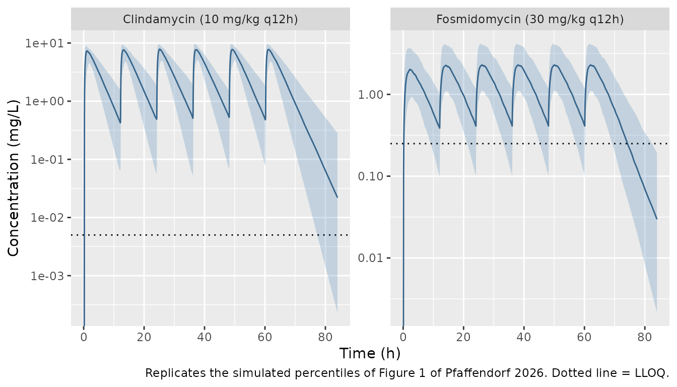
Figure 2 - AUCtau by age group
The paper computes AUCtau as “the AUC over 12 h following the last dose”. The last dose is at 60 h, so the interval is 60-72 h.
TAU_START <- 60   # last of the six q12h doses
TAU_END   <- 72   # one dosing interval later

auctauBy <- function(sim) {
  sim |>
    dplyr::filter(time >= TAU_START, time <= TAU_END) |>
    dplyr::group_by(id, agegrp, WT) |>
    dplyr::summarise(
      # `interval` MUST be given explicitly. pk.calc.auc.last() defaults to
      # interval = c(0, Inf), and on a window that starts at 60 h that is
      # "an AUC range starting (0) before the first measurement (60)", which
      # PKNCA answers with a warning and NA for every subject.
      auctau = PKNCA::pk.calc.auc.last(
        conc = Cc, time = time, interval = c(TAU_START, TAU_END)
      ),
      .groups = "drop"
    )
}
auctauFos <- auctauBy(simFos)
auctauCli <- auctauBy(simCli)
stopifnot(nrow(auctauFos) == 4L * N_PER_ARM, !anyNA(auctauFos$auctau),
          nrow(auctauCli) == 4L * N_PER_ARM, !anyNA(auctauCli$auctau))
# Replicates Figure 2 of Pfaffendorf 2026: AUCtau by age group for
# fosmidomycin 30 mg/kg and clindamycin 10 mg/kg.
dplyr::bind_rows(
  dplyr::mutate(auctauFos, drug = "Fosmidomycin (30 mg/kg)"),
  dplyr::mutate(auctauCli, drug = "Clindamycin (10 mg/kg)")
) |>
  ggplot(aes(agegrp, auctau)) +
  geom_boxplot(fill = "grey85") +
  facet_wrap(~drug, scales = "free_y") +
  labs(x = NULL, y = "AUCtau (mg*h/L)",
       caption = "Replicates Figure 2 of Pfaffendorf 2026.") +
  theme(axis.text.x = element_text(angle = 30, hjust = 1))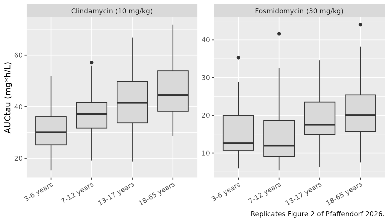
The paper’s two qualitative claims about this figure are that
fosmidomycin exposure is consistent across age groups while clindamycin
exposure is substantially lower in young children. Both follow
structurally from the allometry: dose scales with WT^1 but
clearance with WT^0.75, so AUCtau rises with weight for
both drugs. What differs is that the fosmidomycin spread is dominated by
the large IIV on F and ka, which swamps the allometric trend, while
clindamycin has no IIV on CL/F at all (only 28.8% CV inter-occasion),
leaving the weight trend clearly visible.
medBy <- function(d) {
  m <- d |> dplyr::group_by(agegrp) |>
    dplyr::summarise(med = median(auctau), .groups = "drop")
  stats::setNames(m$med, as.character(m$agegrp))
}
mFos <- medBy(auctauFos)
mCli <- medBy(auctauCli)

# Ratio of the oldest to the youngest age-group median. Asserted as a
# magnitude with generous headroom rather than as an ordering of two noisy
# statistics, so it holds for any cohort the model can draw.
ratFos <- unname(mFos["18-65 years"] / mFos["3-6 years"])
ratCli <- unname(mCli["18-65 years"] / mCli["3-6 years"])

# Structural expectation at the band midpoints: AUCtau ~ Dose/CL ~ WT^0.25.
ratExpect <- ((50 + 86) / 2 / ((12 + 20) / 2))^0.25

# Clindamycin, which has no IIV on CL/F, must track the allometric expectation
# closely. A mis-transcribed exponent (0.75 -> 1, or dropping it) moves this by
# tens of percent and breaks the bound.
stopifnot(abs(ratCli / ratExpect - 1) < 0.15)
# Fosmidomycin carries large IIV on F and ka, so its median ratio is noisier;
# assert only that it is in the same family and well below a doubling.
stopifnot(ratFos > 1.0, ratFos < 2.0)

tibble::tibble(
  Drug      = c("Fosmidomycin", "Clindamycin"),
  `Median AUCtau, 3-6 y`   = c(mFos["3-6 years"],   mCli["3-6 years"]),
  `Median AUCtau, 18-65 y` = c(mFos["18-65 years"], mCli["18-65 years"]),
  `Ratio`   = c(ratFos, ratCli),
  `WT^0.25 expectation` = ratExpect
) |>
  knitr::kable(digits = 2,
caption = "Age-group exposure gradient (Figure 2 of Pfaffendorf 2026).")| Drug | Median AUCtau, 3-6 y | Median AUCtau, 18-65 y | Ratio | WT^0.25 expectation |
|---|---|---|---|---|
| Fosmidomycin | 12.98 | 19.34 | 1.49 | 1.44 |
| Clindamycin | 29.80 | 43.38 | 1.46 | 1.44 |
Figure 3 - the proposed clindamycin dose increase
The paper proposes 12 mg/kg below 35 kg and 10 mg/kg above, implemented as the weight-band table in Additional file 1 S8.
# Replicates Figure 3 of Pfaffendorf 2026: AUCtau under the current 10 mg/kg
# scheme vs the proposed 12-mg/kg-below-35-kg scheme.
subjNew <- dplyr::mutate(subjects, mgkg = ifelse(WT < 35, 12, 10))
dosesNew <- subjNew |>
  tidyr::crossing(time = DOSE_TIMES) |>
  dplyr::mutate(amt = mgkg * WT, evid = 1L, cmt = "depot")
obsNew <- subjNew |>
  tidyr::crossing(time = doseGrid) |>
  dplyr::mutate(amt = NA_real_, evid = 0L, cmt = "central")
evCliNew <- dplyr::bind_rows(dosesNew, obsNew) |>
  dplyr::mutate(OCC = pmin(floor(time / 12) + 1, 6)) |>
  dplyr::arrange(id, time, dplyr::desc(evid))

# Same seed as the 10 mg/kg arm above: common random numbers, so the only
# thing that differs between the two arms is the dose.
rxode2::rxSetSeed(RXSEED)
simCliNew <- rxode2::rxSolve(cliUi, evCliNew, keep = c("agegrp", "WT")) |>
  as.data.frame()
auctauCliNew <- auctauBy(simCliNew)

dplyr::bind_rows(
  dplyr::mutate(auctauCli,    scheme = "Current: 10 mg/kg"),
  dplyr::mutate(auctauCliNew, scheme = "Proposed: 12 mg/kg if <35 kg")
) |>
  ggplot(aes(agegrp, auctau, fill = scheme)) +
  geom_boxplot() +
  labs(x = NULL, y = "Clindamycin AUCtau (mg*h/L)", fill = NULL,
       caption = "Replicates Figure 3 of Pfaffendorf 2026.") +
  theme(axis.text.x = element_text(angle = 30, hjust = 1),
        legend.position = "top")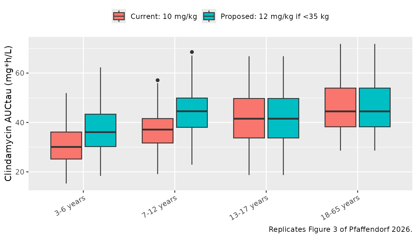
mCliNew <- medBy(auctauCliNew)
# Under common random numbers the two arms differ ONLY in dose, and the model
# is linear in dose, so each subject's AUCtau is scaled by exactly its own
# mg/kg ratio and the band medians scale with it. The 3-6 y and 7-12 y bands
# lie entirely below the 35 kg cut-off (12/10 = 1.2); the 13-17 y and 18-65 y
# bands lie entirely above it (unchanged). These are exact identities, not
# statistical claims, so they are gated to solver tolerance rather than to a
# hand-picked envelope.
expectedRatio <- c("3-6 years" = 1.2, "7-12 years" = 1.2,
                   "13-17 years" = 1.0, "18-65 years" = 1.0)
observedRatio <- mCliNew[names(expectedRatio)] / mCli[names(expectedRatio)]
stopifnot(
  all(abs(observedRatio / expectedRatio - 1) < 1e-6),
  # The band/cut-off assumption the identity rests on, asserted rather than
  # assumed: no subject straddles its band's side of the 35 kg cut-off.
  all(subjects$WT[subjects$agegrp %in% c("3-6 years", "7-12 years")] < 35),
  all(subjects$WT[subjects$agegrp %in% c("13-17 years", "18-65 years")] >= 35)
)
# ... and it narrows the spread of medians across age groups, which is the
# paper's stated purpose ("more uniform drug exposure across age groups").
spreadOld <- max(mCli) / min(mCli)
spreadNew <- max(mCliNew) / min(mCliNew)
stopifnot(spreadNew < spreadOld)

tibble::tibble(
  `Age group`        = names(mCli),
  `Current 10 mg/kg` = as.numeric(mCli),
  `Proposed scheme`  = as.numeric(mCliNew[names(mCli)]),
  `Ratio`            = as.numeric(mCliNew[names(mCli)]) / as.numeric(mCli)
) |>
  knitr::kable(digits = 2,
caption = "Median clindamycin AUCtau under the current and proposed dosing.")| Age group | Current 10 mg/kg | Proposed scheme | Ratio |
|---|---|---|---|
| 3-6 years | 29.80 | 35.76 | 1.2 |
| 7-12 years | 36.12 | 43.34 | 1.2 |
| 13-17 years | 38.80 | 38.80 | 1.0 |
| 18-65 years | 43.38 | 43.38 | 1.0 |
The S8 weight bands are reproduced here for reference; the model
file’s population$dose_range carries the same table.
tibble::tribble(
  ~`Clindamycin dose (mg)`, ~`Weight range (kg)`,
  150, "<18.7",
  300, "18.7-31.2",
  450, "31.2-52.5",
  600, "52.5-67.5",
  750, "67.5-82.5",
  900, "82.5-97.5"
) |>
knitr::kable(caption = "Additional file 1 S8: proposed clindamycin weight bands.")| Clindamycin dose (mg) | Weight range (kg) |
|---|---|
| 150 | <18.7 |
| 300 | 18.7-31.2 |
| 450 | 31.2-52.5 |
| 600 | 52.5-67.5 |
| 750 | 67.5-82.5 |
| 900 | 82.5-97.5 |
PKNCA validation
One PKNCA block per drug. AUCtau is taken over the last dosing interval (60-72 h) and the terminal half-life over the washout window after the last dose (72-96 h).
runNca <- function(sim, ev) {
  conc <- sim |>
    dplyr::filter(!is.na(Cc)) |>
    dplyr::select(id, time, Cc, agegrp)
  # Guarantee a time = 0 row per subject; for extravascular dosing Cc = 0
  # pre-dose is correct, and its absence triggers PKNCA's "AUC range starting
  # before the first measurement" warning on every subject.
  conc <- dplyr::bind_rows(
    conc,
    conc |> dplyr::distinct(id, agegrp) |> dplyr::mutate(time = 0, Cc = 0)
  ) |>
    dplyr::distinct(id, agegrp, time, .keep_all = TRUE) |>
    dplyr::arrange(id, time)

  concObj <- PKNCA::PKNCAconc(conc, Cc ~ time | agegrp + id)

  doseDf <- ev |>
    dplyr::filter(evid == 1) |>
    dplyr::select(id, time, amt, agegrp)
  doseObj <- PKNCA::PKNCAdose(doseDf, amt ~ time | agegrp + id)

  intervals <- data.frame(
    start     = c(60, 72),
    end       = c(72, 96),
    cmax      = c(TRUE,  FALSE),
    tmax      = c(TRUE,  FALSE),
    auclast   = c(TRUE,  FALSE),
    half.life = c(FALSE, TRUE)
  )
  PKNCA::pk.nca(PKNCA::PKNCAdata(concObj, doseObj, intervals = intervals))
}

ncaFos <- runNca(simFos, evFosPop)
ncaCli <- runNca(simCli, evCliPop)

ncaSummary <- function(res, drug) {
  as.data.frame(res) |>
    dplyr::filter(PPTESTCD %in% c("cmax", "tmax", "auclast", "half.life")) |>
    dplyr::group_by(agegrp, PPTESTCD) |>
    dplyr::summarise(median = median(PPORRES, na.rm = TRUE), .groups = "drop") |>
    dplyr::mutate(drug = drug)
}
ncaTab <- dplyr::bind_rows(ncaSummary(ncaFos, "Fosmidomycin"),
                           ncaSummary(ncaCli, "Clindamycin"))
stopifnot(nrow(ncaTab) > 0L, !all(is.na(ncaTab$median)))

ncaTab |>
  tidyr::pivot_wider(names_from = PPTESTCD, values_from = median) |>
  dplyr::relocate(drug, agegrp) |>
  dplyr::rename(
    "Drug"                = drug,
    "Age group"           = agegrp,
    "Cmax (mg/L)"         = cmax,
    # PKNCA reports tmax on the simulation clock, so within the 60-72 h
    # interval it reads as 60 + the true time to peak.
    "Tmax (h, clock time)" = tmax,
    "AUCtau (mg*h/L)"     = auclast,
    "t1/2 (h)"            = half.life
  ) |>
  knitr::kable(digits = 3,
caption = "Simulated steady-state NCA by drug and age group (medians).")| Drug | Age group | AUCtau (mg*h/L) | Cmax (mg/L) | t1/2 (h) | Tmax (h, clock time) |
|---|---|---|---|---|---|
| Fosmidomycin | 3-6 years | 12.982 | 1.908 | 2.768 | 0.575 |
| Fosmidomycin | 7-12 years | 14.960 | 2.260 | 3.153 | 0.275 |
| Fosmidomycin | 13-17 years | 14.698 | 2.040 | 3.345 | 0.550 |
| Fosmidomycin | 18-65 years | 19.343 | 2.487 | 3.836 | 0.600 |
| Clindamycin | 3-6 years | 29.796 | 7.067 | 1.976 | 0.250 |
| Clindamycin | 7-12 years | 36.119 | 7.726 | 2.359 | 0.150 |
| Clindamycin | 13-17 years | 38.795 | 7.976 | 2.681 | 0.250 |
| Clindamycin | 18-65 years | 43.385 | 8.378 | 2.910 | 0.325 |
Comparison against published NCA
Pfaffendorf 2026 reports no NCA table. The quantitative statements it does make are the two terminal half-lives and the clindamycin exposure range, both in the Discussion. Those are the reference values below; because the paper gives the clindamycin exposure as a range (“our median exposure of approximately 30-40 mg h/L”), its midpoint 35 mg*h/L is used as the point of comparison.
simForCmp <- tibble::tibble(
  drug     = c("Fosmidomycin", "Clindamycin", "Clindamycin"),
  PPTESTCD = c("half.life", "half.life", "auclast"),
  PPORRES  = c(
    hlFos,
    hlCli,
    median(auctauCli$auctau)
  )
)
published <- tibble::tribble(
  ~drug,           ~half.life, ~auclast,
  "Fosmidomycin",  2.9,        NA_real_,
  "Clindamycin",   2.5,        35.0
)

cmp <- nlmixr2lib::ncaComparisonTable(
  simulated = simForCmp,
  reference = published,
  by        = "drug",
  units     = c(half.life = "h", auclast = "mg*h/L"),
  tolerance_pct = 20
)
knitr::kable(cmp, caption = "Simulated vs. published. * differs by >20%.",
align = c("l", "l", "r", "r", "r"))| NCA parameter | drug | Reference | Simulated | % diff |
|---|---|---|---|---|
| AUClast (mg*h/L) | Clindamycin | 35 | 37.3 | +6.6% |
| t½ (h) | Fosmidomycin | 2.9 | 2.96 | +2.1% |
| t½ (h) | Clindamycin | 2.5 | 2.46 | -1.8% |
attr(cmp, "footnote")
#> NULL
# Half-lives are deterministic typical-value quantities (zeroRe), so they are
# gated tightly. The clindamycin exposure is a cohort median compared against
# the midpoint of a range the paper states to one significant figure, so it is
# gated only against the stated range itself.
medCliAuc <- median(auctauCli$auctau)
stopifnot(
  abs(hlFos - 2.9) < 0.1,
  abs(hlCli - 2.5) < 0.1,
  medCliAuc >= 30, medCliAuc <= 40
)
The simulated clindamycin AUCtau median of 37.3 mgh/L sits inside
the 30-40 mgh/L the Discussion reports, and equals
Dose/CL at the reference subject (36.2 mg*h/L) to within
the cohort’s weight spread, as it must for a linear model with F fixed
at 1.
Assumptions and deviations
- Weight distribution per age group. The paper sampled weights “from a normal distribution, using the age-specific means and standard deviations observed in the study population”, but those per-group means and SDs are not published. This vignette instead samples uniformly within the weight bands that the paper itself ties to the age groups (cut-offs 20, 35, 50 kg; Results / Clindamycin dosing simulation), bounded by the observed cohort range 12.0-86.0 kg (Table 1). Exposure medians therefore reproduce the published trend across age groups, not the exact published quartiles.
- Body temperature is drawn from N(37.1, 1.06) (Table 1) truncated to the observed 35.4-39.0 degC range. The paper explicitly cautions against extrapolating the temperature effect outside the measured range, and the exponent 6.68 makes the term very steep, so truncation is a deliberate guard rather than a convenience.
-
Body temperature is treated as time-fixed at its
admission value. The paper notes temperature was measured only twice
daily and that “these discrete measurements do not capture the complete
temporal profile”; the control stream carries
BTas a data column, so a time-varyingBODYTEMPcolumn is equally valid input to the packaged model. - Doses are exact mg/kg. The trial rounded each dose “to the closest possible match using the available formulations” (75 / 225 / 450 mg fosmidomycin capsules; 150 / 300 / 600 mg clindamycin). Rounding is not reproduced here, so simulated exposures are marginally smoother than observed.
-
Zero-variance etas are omitted, not encoded as
fixed(0). Fosmidomycin’s$OMEGA 1(IIV on V) and clindamycin’s$OMEGA 1-3(IIV on CL, Vc, F1) are all0 FIXin the final control streams, and Table 2 reports no omega row for any of them. A zero-variance diagonal makes OMEGA singular and breaks the Cholesky samplerrxSolveuses, so those etas are simply absent from the model files. The simulated variability is unchanged; only the eta bookkeeping differs from the NONMEM listing. -
Clindamycin has no IIV on clearance at all. All
between-occasion variability in clindamycin CL/F is carried by the
six-occasion IOV term (28.8% CV).
OCCmust be supplied in the event table; for a single-dose or single-occasion simulation passOCC = 1. - Body-temperature effect magnitude (deviation, not gated). The Discussion states the model “predicts a 60% increase in clearance at a body temperature of 40 degC”. Evaluating the published relationship exactly gives `(40/37.1)^6.68 = 1.653, a 65% increase. The model file reproduces the control stream verbatim, so the difference is in the paper’s one-significant -figure narrative rounding, not in the implementation.
- No observed data. Figure 1 of the paper is a reference-corrected VPC against observed concentrations; only the simulated percentile bands can be reproduced here. Likewise the paper reports no NCA table, so the comparison section is limited to the two Discussion half-lives and the clindamycin exposure range.
- Artesunate was co-administered in the trial but was not modelled by this paper (it was the subject of a different arm), so it is absent from both model files. The paper notes that a CYP3A4-induction interaction with clindamycin is theoretically possible but that observed exposures were comparable to prior studies without artesunate.