Transdermal caffeine and anti-inflammatory drugs in a skin-on-a-chip chamber (Szederkenyi 2024)
Source:vignettes/articles/Szederkenyi_2024_transdermal_skinonachip.Rmd
Szederkenyi_2024_transdermal_skinonachip.RmdModel and source
- Citation: Szederkenyi G, Kocsis D, Vaghy MA, Czaran D, Sasvari P, Lengyel M, Naszlady MB, Kreis F, Antal I, Csepanyi-Komi R, Erdo F. Mathematical modeling of transdermal delivery of topical drug formulations in a dynamic microfluidic diffusion chamber in health and disease. PLoS One. 2024;19(4):e0299501. doi:10.1371/journal.pone.0299501. PMCID: PMC11008853. Model: Section 2.7, Eq 1; estimates: S1 Table (row ‘caffeine 6hr’); fit: Figure 4A.
- Article: https://doi.org/10.1371/journal.pone.0299501
- Supplement (S1 Table, parameter estimates): https://doi.org/10.1371/journal.pone.0299501.s001
Szederkenyi et al. measured the penetration of topically applied 2%
O/W creams through excised skin mounted in a dynamic “skin-on-a-chip”
microfluidic diffusion chamber, and described every measured
cumulative-permeation curve with the same three-compartment linear ODE
model (Section 2.7, Eq 1). The three compartments are the layers of the
skin obtained by spatially discretising a diffusion-convection equation:
a constant zero-order input kin from the cream enters the
outermost layer, neighbouring layers exchange drug by diffusion
(kd, both directions) and by inward convection
(kc), and the deepest layer loses drug at the first-order
rate kout. The only observed quantity is the deepest-layer
state, y = x3, which the authors fit to the cumulative drug
mass permeated into the receptor fluid per cm^2 of diffusion
surface.
The model was fitted separately to each experiment’s mean curve, giving 13 independent parameter sets (S1 Table). nlmixr2lib ships each as its own model:
cases <- tibble::tribble(
  ~model,                                    ~experiment,                                ~figure,  ~tend, ~mass_unit,
  "Szederkenyi_2024_caffeine_rt6h",          "Caffeine, rat skin, 23.5 C, 6 h",          "4A",     6,     "ug/cm^2",
  "Szederkenyi_2024_caffeine_32c6h",         "Caffeine, rat skin, 32 C, 6 h",            "4B",     6,     "ug/cm^2",
  "Szederkenyi_2024_caffeine_rt12h",         "Caffeine, rat skin, 23.5 C, 12 h",         "5",      12,    "ug/cm^2",
  "Szederkenyi_2024_dexamethasone",          "Dexamethasone acetate, rat skin",          "6A",     6,     "ng/cm^2",
  "Szederkenyi_2024_piroxicam",              "Piroxicam, rat skin",                      "6B",     6,     "ng/cm^2",
  "Szederkenyi_2024_indomethacin",           "Indomethacin, rat skin",                   "6C",     6,     "ng/cm^2",
  "Szederkenyi_2024_diclofenac",             "Diclofenac, rat skin",                     "6D",     6,     "ug/cm^2",
  "Szederkenyi_2024_caffeine_vaseline24h",   "Caffeine, mouse skin, vaseline 24 h",      "8A",     5,     "ug/cm^2",
  "Szederkenyi_2024_caffeine_vaseline96h",   "Caffeine, mouse skin, vaseline 96 h",      "8B",     5,     "ug/cm^2",
  "Szederkenyi_2024_caffeine_imiquimod24h",  "Caffeine, mouse skin, imiquimod 24 h",     "8C",     5,     "ug/cm^2",
  "Szederkenyi_2024_caffeine_imiquimod96h",  "Caffeine, mouse skin, imiquimod 96 h",     "8D",     5,     "ug/cm^2",
  "Szederkenyi_2024_caffeine_ear_acetone",   "Caffeine, mouse ear, acetone control",     "10A",    5,     "ug/cm^2",
  "Szederkenyi_2024_caffeine_ear_tncb",      "Caffeine, mouse ear, TNCB allergic",       "10B",    5,     "ug/cm^2"
)
uis <- lapply(cases$model, function(nm) rxode2::rxode(readModelDb(nm)))
names(uis) <- cases$model
knitr::kable(cases |> dplyr::select(model, experiment, figure))| model | experiment | figure |
|---|---|---|
| Szederkenyi_2024_caffeine_rt6h | Caffeine, rat skin, 23.5 C, 6 h | 4A |
| Szederkenyi_2024_caffeine_32c6h | Caffeine, rat skin, 32 C, 6 h | 4B |
| Szederkenyi_2024_caffeine_rt12h | Caffeine, rat skin, 23.5 C, 12 h | 5 |
| Szederkenyi_2024_dexamethasone | Dexamethasone acetate, rat skin | 6A |
| Szederkenyi_2024_piroxicam | Piroxicam, rat skin | 6B |
| Szederkenyi_2024_indomethacin | Indomethacin, rat skin | 6C |
| Szederkenyi_2024_diclofenac | Diclofenac, rat skin | 6D |
| Szederkenyi_2024_caffeine_vaseline24h | Caffeine, mouse skin, vaseline 24 h | 8A |
| Szederkenyi_2024_caffeine_vaseline96h | Caffeine, mouse skin, vaseline 96 h | 8B |
| Szederkenyi_2024_caffeine_imiquimod24h | Caffeine, mouse skin, imiquimod 24 h | 8C |
| Szederkenyi_2024_caffeine_imiquimod96h | Caffeine, mouse skin, imiquimod 96 h | 8D |
| Szederkenyi_2024_caffeine_ear_acetone | Caffeine, mouse ear, acetone control | 10A |
| Szederkenyi_2024_caffeine_ear_tncb | Caffeine, mouse ear, TNCB allergic | 10B |
Population
There is no human or animal population in the usual sense: each model describes the mean of three replicate skin samples (n = 3 per experiment, figure captions) in one ex vivo set-up. The chamber has a 0.5 cm^2 diffusion surface between the cream-filled donor chamber and a receptor chamber perfused with peripheral perfusion fluid (147 mM NaCl, 4 mM KCl, 2.3 mM CaCl2, pH 7.4) at 4 uL/min; receptor fluid was collected every 30 or 15 min (Section 2.4).
- Healthy-skin experiments (caffeine at room temperature and at 32 C, and the four anti-inflammatory creams) used tape-stripped abdominal skin of rats weighing 599-615 g (Sections 2.4 and 2.6).
- Psoriasiform dermatitis was induced in male C57BL/6J mice (21.7-27.0 g) with 0.0625 g of 5% imiquimod cream on the shaved back (once for the 24 h group, daily for the 96 h group), with vaseline-treated time-matched controls (Section 2.5).
- Allergic contact dermatitis was induced in male C57BL/6J mice (24.2-31.2 g) by sensitising the abdomen with 3% TNCB (controls: acetone) and challenging both ears with 1% TNCB on day 5; the ear tissue was mounted in the chamber (Section 2.5).
Caffeine was assayed by NanoDrop spectrophotometry at 273 nm and the
anti-inflammatory drugs by LC-MS/MS. The same information is stored in
each model’s population metadata:
str(uis[["Szederkenyi_2024_caffeine_rt6h"]]$population)
#> List of 11
#>  $ species      : chr "ex vivo (rat abdominal skin)"
#>  $ n_subjects   : int 3
#>  $ n_studies    : int 1
#>  $ system       : chr "Skin-on-a-chip microfluidic diffusion chamber (polydimethylsiloxane in an aluminium frame): a 0.5 cm^2 diffusio"| __truncated__
#>  $ tissue       : chr "Full-thickness 18-mm punches of shaved, depilated and tape-stripped (10 strips) abdominal skin of rats weighing"| __truncated__
#>  $ dose_range   : chr "O/W cream (46% petrolatum basis ointment, 4% paraffin oil, 38% purified water, 10% propylene glycol) containing"| __truncated__
#>  $ temperature  : chr "room temperature, approximately 23.5 C (air-conditioned laboratory)"
#>  $ sampling     : chr "Receptor fluid collected every 30 or 15 min for 6 h; caffeine in the collected receptor fluid by NanoDrop spect"| __truncated__
#>  $ disease_state: chr "healthy (intact skin)"
#>  $ regions      : chr "Hungary (Budapest)"
#>  $ notes        : chr "Mean of n = 3 replicate skin samples (Figure 4A caption); the model was fitted to the mean curve by minimising "| __truncated__
Source trace
Every ini() value carries an in-file comment pointing to
its row of S1 Table. All four parameters were estimated (Matlab
fmincon, Eq 7) on the linear scale and are reported without
uncertainty; nlmixr2lib stores them log-transformed.
| Model element | Source location |
|---|---|
d/dt(skin_slab1), d/dt(skin_slab2),
d/dt(skin_slab3)
|
Section 2.7, Eq 1 (states x1, x2,
x3) |
Output cum_mass <- skin_slab3
|
Section 2.7 (“The only measured concentration is y = x3”); figure y-axes (cumulative mass per cm^2) |
lkin, lkdiff, lkconv,
lkout (paper kin, kd,
kc, kout) |
S1 Table, one row per model |
| Zero initial conditions | Figures 4-10 (all simulated curves start at 0); S1 Table reports no initial-condition estimates |
| Time unit (h) | Figure x-axes |
| Mass units (ug/cm^2 or ng/cm^2) | Figure y-axes; Table 2 |
s1 <- dplyr::bind_rows(lapply(cases$model, function(nm) {
  th <- uis[[nm]]$theta
  tibble::tibble(
    model = nm,
    kin = exp(th[["lkin"]]),
    kd = exp(th[["lkdiff"]]),
    kc = exp(th[["lkconv"]]),
    kout = exp(th[["lkout"]])
  )
}))
knitr::kable(s1, digits = 6, caption = "Back-transformed parameters (compare S1 Table).")| model | kin | kd | kc | kout |
|---|---|---|---|---|
| Szederkenyi_2024_caffeine_rt6h | 7.4371 | 0.033600 | 3.37780 | 0.029300 |
| Szederkenyi_2024_caffeine_32c6h | 11.8667 | 0.031900 | 3.66370 | 0.019300 |
| Szederkenyi_2024_caffeine_rt12h | 9.2316 | 0.019800 | 2.04090 | 0.000042 |
| Szederkenyi_2024_dexamethasone | 874.9814 | 0.000034 | 0.22190 | 0.000039 |
| Szederkenyi_2024_piroxicam | 821.8726 | 0.000012 | 0.37762 | 0.000016 |
| Szederkenyi_2024_indomethacin | 111.8016 | 0.000646 | 0.26900 | 0.000643 |
| Szederkenyi_2024_diclofenac | 52.0705 | 0.027900 | 0.36810 | 0.223100 |
| Szederkenyi_2024_caffeine_vaseline24h | 3.6499 | 0.120600 | 30.64610 | 0.336500 |
| Szederkenyi_2024_caffeine_vaseline96h | 3.1878 | 0.215000 | 261.08480 | 0.220700 |
| Szederkenyi_2024_caffeine_imiquimod24h | 10.0399 | 0.027200 | 3.13610 | 0.000304 |
| Szederkenyi_2024_caffeine_imiquimod96h | 7.5925 | 0.063700 | 7.40990 | 0.000035 |
| Szederkenyi_2024_caffeine_ear_acetone | 0.5846 | 1.849400 | 1017.20590 | 0.000738 |
| Szederkenyi_2024_caffeine_ear_tncb | 1.1352 | 0.034700 | 9.06110 | 0.123600 |
Simulation
The models carry no between-sample variability and no residual error,
so each is solved once at its typical values. There are no dose records:
the cream is the constant input kin.
sim <- dplyr::bind_rows(lapply(seq_len(nrow(cases)), function(i) {
  ev <- rxode2::et(seq(0, cases$tend[i], by = 0.05))
  s <- rxode2::rxSolve(uis[[cases$model[i]]], events = ev, rtol = 1e-10, atol = 1e-12)
  tibble::tibble(
    model = cases$model[i],
    experiment = cases$experiment[i],
    figure = cases$figure[i],
    mass_unit = cases$mass_unit[i],
    time = s$time,
    cum_mass = s$cum_mass
  )
}))
Replicate published figures
plot_cases <- function(figs, title) {
  sim |>
    dplyr::filter(figure %in% figs) |>
    dplyr::mutate(panel = paste0("Fig ", figure, ": ", experiment, " (", mass_unit, ")")) |>
    ggplot(aes(time, cum_mass)) +
    geom_line(colour = "red") +
    facet_wrap(~panel, scales = "free_y") +
    labs(x = "Time (h)", y = "Cumulative mass permeated per cm^2", title = title)
}
plot_cases(c("4A", "4B", "5"), "Caffeine through healthy rat skin") +
  labs(caption = "Replicates the simulated curves of Figures 4A, 4B and 5 of Szederkenyi 2024.")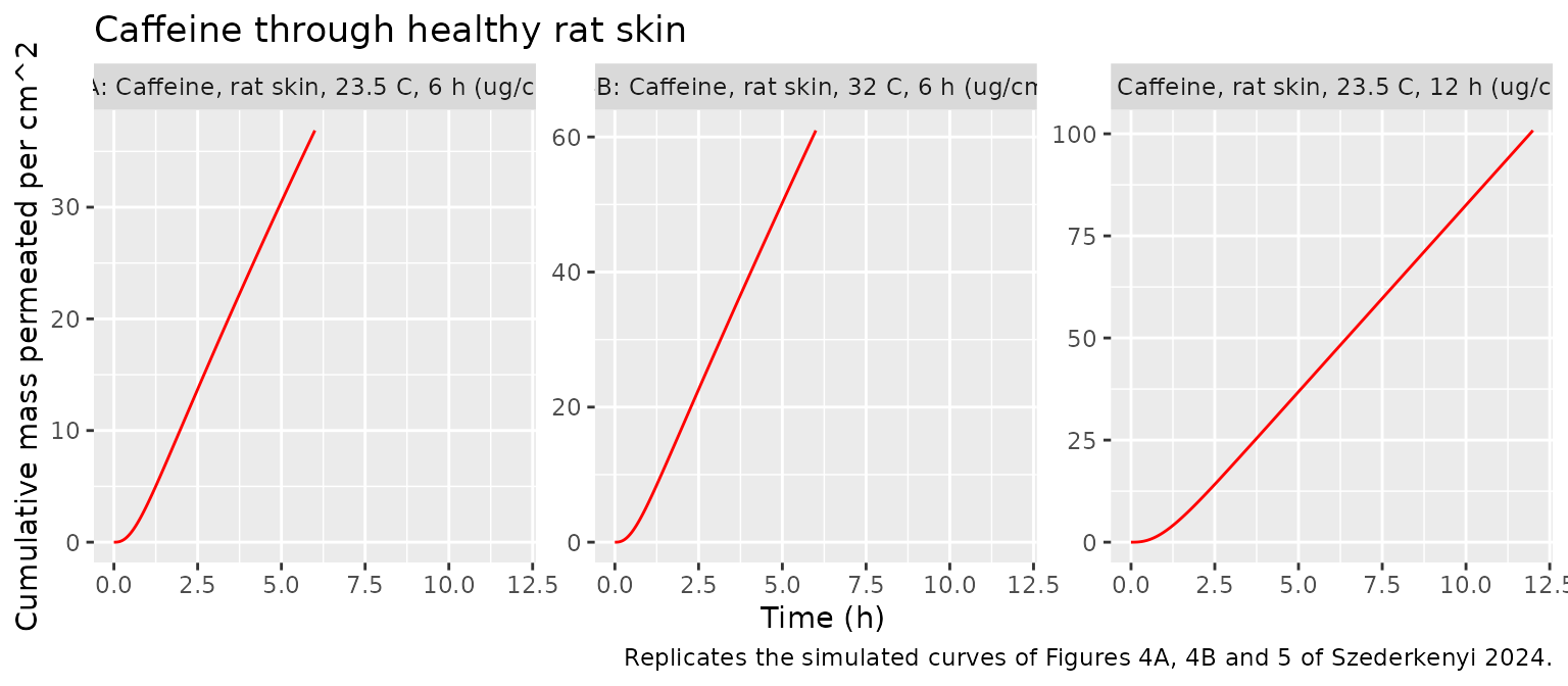
plot_cases(c("6A", "6B", "6C", "6D"), "Anti-inflammatory creams through rat skin") +
  labs(caption = "Replicates the simulated curves of Figure 6 of Szederkenyi 2024.")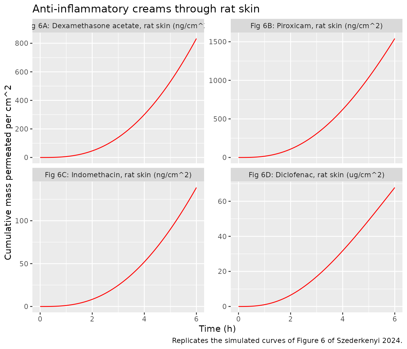
plot_cases(c("8A", "8B", "8C", "8D"), "Caffeine through control and psoriatic mouse skin") +
  labs(caption = "Replicates the simulated curves of Figure 8 of Szederkenyi 2024.")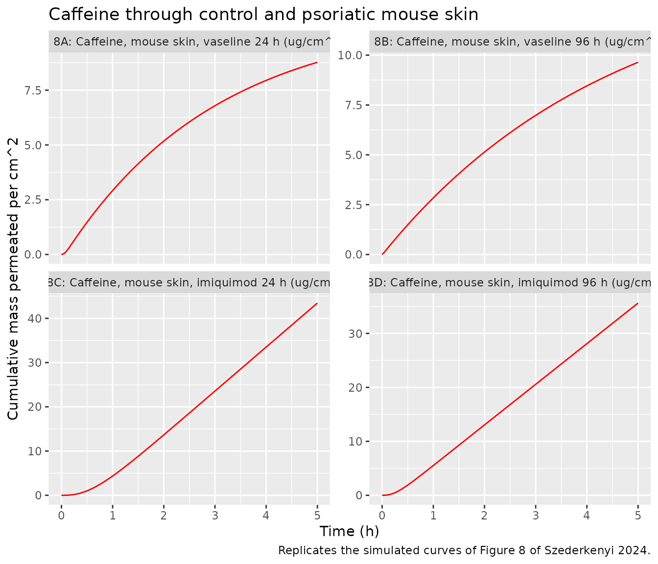
plot_cases(c("10A", "10B"), "Caffeine through control and allergic mouse ear tissue") +
  labs(caption = "Replicates the simulated curves of Figure 10 of Szederkenyi 2024.")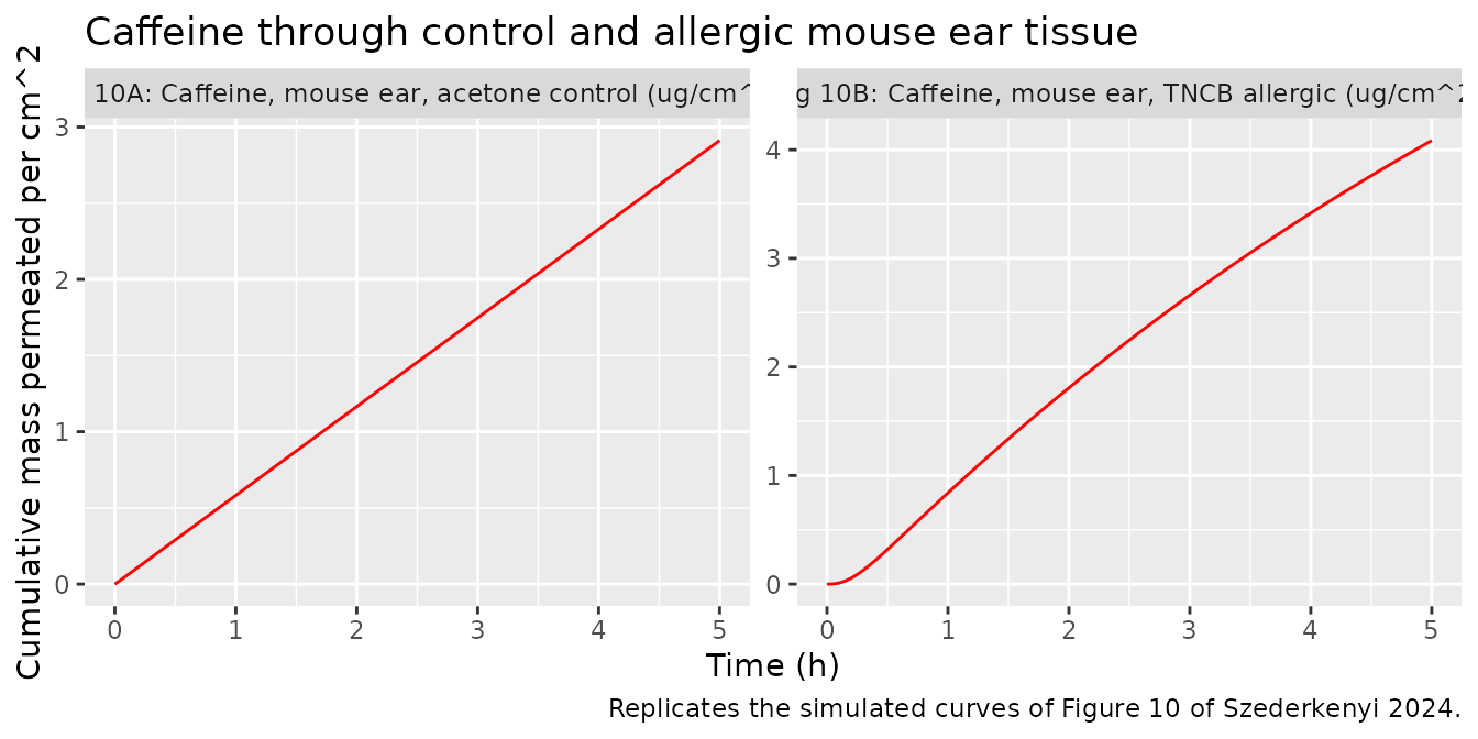
Validation
The paper reports no NCA, so PKNCA does not apply. The checks below compare the packaged models against the printed numbers that the paper does give, and against the closed-form solution of Eq 1.
Final cumulative mass against the published curves
The final value of each red simulated curve in Figures 4, 5, 6, 8 and 10 was read off the figure by the maintainers (precision about 2-3% of the axis range). The packaged models reproduce every one within 5%.
digitised <- tibble::tribble(
  ~figure, ~fig_end,
  "4A",    37.0,
  "4B",    61.0,
  "5",     101,
  "6A",    830,
  "6B",    1560,
  "6C",    140,
  "6D",    67.5,
  "8A",    8.75,
  "8B",    9.65,
  "8C",    43.3,
  "8D",    35.5,
  "10A",   2.90,
  "10B",   4.08
)
final <- sim |>
  dplyr::group_by(model, figure, mass_unit) |>
  dplyr::filter(time == max(time)) |>
  dplyr::ungroup() |>
  dplyr::select(model, figure, mass_unit, time, cum_mass) |>
  dplyr::inner_join(digitised, by = "figure") |>
  dplyr::mutate(pct_diff = 100 * (cum_mass / fig_end - 1))
stopifnot(nrow(final) == nrow(cases), all(abs(final$pct_diff) < 5))
final |>
  dplyr::rename(
    "Figure" = figure,
    "Units" = mass_unit,
    "Time (h)" = time,
    "Simulated" = cum_mass,
    "Published (figure)" = fig_end,
    "Difference (%)" = pct_diff
  ) |>
knitr::kable(digits = 2)| model | Figure | Units | Time (h) | Simulated | Published (figure) | Difference (%) |
|---|---|---|---|---|---|---|
| Szederkenyi_2024_caffeine_rt6h | 4A | ug/cm^2 | 6 | 36.87 | 37.00 | -0.34 |
| Szederkenyi_2024_caffeine_32c6h | 4B | ug/cm^2 | 6 | 60.96 | 61.00 | -0.06 |
| Szederkenyi_2024_caffeine_rt12h | 5 | ug/cm^2 | 12 | 100.82 | 101.00 | -0.18 |
| Szederkenyi_2024_dexamethasone | 6A | ng/cm^2 | 6 | 833.04 | 830.00 | 0.37 |
| Szederkenyi_2024_piroxicam | 6B | ng/cm^2 | 6 | 1541.58 | 1560.00 | -1.18 |
| Szederkenyi_2024_indomethacin | 6C | ng/cm^2 | 6 | 138.70 | 140.00 | -0.93 |
| Szederkenyi_2024_diclofenac | 6D | ug/cm^2 | 6 | 67.82 | 67.50 | 0.47 |
| Szederkenyi_2024_caffeine_vaseline24h | 8A | ug/cm^2 | 5 | 8.77 | 8.75 | 0.25 |
| Szederkenyi_2024_caffeine_vaseline96h | 8B | ug/cm^2 | 5 | 9.64 | 9.65 | -0.10 |
| Szederkenyi_2024_caffeine_imiquimod24h | 8C | ug/cm^2 | 5 | 43.45 | 43.30 | 0.34 |
| Szederkenyi_2024_caffeine_imiquimod96h | 8D | ug/cm^2 | 5 | 35.62 | 35.50 | 0.34 |
| Szederkenyi_2024_caffeine_ear_acetone | 10A | ug/cm^2 | 5 | 2.91 | 2.90 | 0.39 |
| Szederkenyi_2024_caffeine_ear_tncb | 10B | ug/cm^2 | 5 | 4.08 | 4.08 | 0.12 |
Table 2 acceptance windows
Table 2 lists the a-posteriori acceptance window for the measured cumulative mass at the end of each healthy-skin experiment; replicates outside it were excluded before fitting. A faithful fit to the mean of the accepted replicates must end inside the window.
table2 <- tibble::tribble(
  ~model,                             ~lower, ~upper,
  "Szederkenyi_2024_caffeine_rt6h",   20,     50,
  "Szederkenyi_2024_caffeine_32c6h",  40,     75,
  "Szederkenyi_2024_caffeine_rt12h",  80,     120,
  "Szederkenyi_2024_dexamethasone",   600,    1000,
  "Szederkenyi_2024_indomethacin",    100,    200,
  "Szederkenyi_2024_piroxicam",       1200,   2000,
  "Szederkenyi_2024_diclofenac",      50,     100
)
t2 <- final |>
  dplyr::select(model, mass_unit, cum_mass) |>
  dplyr::inner_join(table2, by = "model")
stopifnot(nrow(t2) == 7, all(t2$cum_mass > t2$lower & t2$cum_mass < t2$upper))
knitr::kable(t2, digits = 1)| model | mass_unit | cum_mass | lower | upper |
|---|---|---|---|---|
| Szederkenyi_2024_caffeine_rt6h | ug/cm^2 | 36.9 | 20 | 50 |
| Szederkenyi_2024_caffeine_32c6h | ug/cm^2 | 61.0 | 40 | 75 |
| Szederkenyi_2024_caffeine_rt12h | ug/cm^2 | 100.8 | 80 | 120 |
| Szederkenyi_2024_dexamethasone | ng/cm^2 | 833.0 | 600 | 1000 |
| Szederkenyi_2024_piroxicam | ng/cm^2 | 1541.6 | 1200 | 2000 |
| Szederkenyi_2024_indomethacin | ng/cm^2 | 138.7 | 100 | 200 |
| Szederkenyi_2024_diclofenac | ug/cm^2 | 67.8 | 50 | 100 |
Disease effects stated in the text
Section 3.5 states that imiquimod raised the caffeine permeability “more than 4 times at 24 h, and more than 3.5 times at 96 h” over the time-matched vaseline controls; Section 3.6 states that allergic contact dermatitis raised the ear permeability by 30%.
end_of <- function(nm) final$cum_mass[final$model == nm]
ratios <- tibble::tibble(
  comparison = c("Imiquimod / vaseline, 24 h", "Imiquimod / vaseline, 96 h", "TNCB / acetone (ear)"),
  simulated_ratio = c(
    end_of("Szederkenyi_2024_caffeine_imiquimod24h") / end_of("Szederkenyi_2024_caffeine_vaseline24h"),
    end_of("Szederkenyi_2024_caffeine_imiquimod96h") / end_of("Szederkenyi_2024_caffeine_vaseline96h"),
    end_of("Szederkenyi_2024_caffeine_ear_tncb") / end_of("Szederkenyi_2024_caffeine_ear_acetone")
  ),
  paper = c("> 4", "> 3.5", "1.3")
)
stopifnot(
  ratios$simulated_ratio[1] > 4,
  ratios$simulated_ratio[2] > 3.5,
  ratios$simulated_ratio[3] > 1
)
knitr::kable(ratios, digits = 2)| comparison | simulated_ratio | paper |
|---|---|---|
| Imiquimod / vaseline, 24 h | 4.95 | > 4 |
| Imiquimod / vaseline, 96 h | 3.70 | > 3.5 |
| TNCB / acetone (ear) | 1.40 | 1.3 |
The imiquimod ratios meet the stated thresholds. The ear ratio from the fitted curves at 5 h is about 1.4 rather than the stated 1.3; the measured curves of Figure 10 end at about 2.95 and 4.1 ug/cm^2, also a ratio near 1.4, so the paper’s 30% presumably comes from a different summary (for example the permeation rate over part of the experiment) that is not reported.
Closed-form solution and the eliminated model (Eqs 2-6)
Eq 1 is linear, x' = A x + b with
b = (kin, 0, 0) and zero initial state, so
x(t) = A^-1 (exp(A t) - I) b. The packaged ODE must match
this to integration precision. The authors’ identifiability argument
rewrites the model as
y''' + theta1 y'' + theta2 y' + theta3 y + theta4 = 0 (Eqs
2-6); theta1..theta3 are the characteristic-polynomial
coefficients of A, and the steady state of y
is -theta4 / theta3 = kin / kout. Both identities are
checked for every parameter set.
system_matrix <- function(kd, kc, kout) {
  matrix(c(
    -(kd + kc), kd, 0,
    kd + kc, -(2 * kd + kc), kd,
    0, kd + kc, -(kd + kout)
  ), nrow = 3, byrow = TRUE)
}
x3_closed_form <- function(times, kin, kd, kc, kout) {
  A <- system_matrix(kd, kc, kout)
  e <- eigen(A)
  vinv <- solve(e$vectors)
  b <- c(kin, 0, 0)
  vapply(times, function(t) {
    expAt <- Re(e$vectors %*% diag(exp(e$values * t)) %*% vinv)
    (solve(A, (expAt - diag(3)) %*% b))[3]
  }, numeric(1))
}
cf <- dplyr::bind_rows(lapply(seq_len(nrow(s1)), function(i) {
  p <- s1[i, ]
  s <- sim[sim$model == p$model, ]
  A <- system_matrix(p$kd, p$kc, p$kout)
  minors <- A[1, 1] * A[2, 2] - A[1, 2] * A[2, 1] +
    A[2, 2] * A[3, 3] - A[2, 3] * A[3, 2] +
    A[1, 1] * A[3, 3] - A[1, 3] * A[3, 1]
  theta <- c(
    2 * p$kc + 4 * p$kd + p$kout,
    p$kc^2 + 3 * p$kc * p$kd + 2 * p$kout * p$kc + 3 * p$kd^2 + 3 * p$kout * p$kd,
    p$kout * p$kc^2 + 2 * p$kout * p$kc * p$kd + p$kout * p$kd^2,
    -p$kin * (p$kc + p$kd)^2
  )
  tibble::tibble(
    model = p$model,
    ode_vs_closed_form = max(abs(s$cum_mass - x3_closed_form(s$time, p$kin, p$kd, p$kc, p$kout))) /
      max(s$cum_mass),
    theta_vs_charpoly = max(abs(c(-sum(diag(A)), minors, -det(A)) / theta[1:3] - 1)),
    steady_state = -theta[4] / theta[3],
    steady_state_vs_kin_over_kout = abs(-theta[4] / theta[3] / (p$kin / p$kout) - 1)
  )
}))
# The ODE-vs-closed-form error is integration error at rtol = 1e-10; the
# theta and steady-state identities are pure floating-point algebra.
stopifnot(
  all(cf$ode_vs_closed_form < 1e-6),
  all(cf$theta_vs_charpoly < 1e-10),
  all(cf$steady_state_vs_kin_over_kout < 1e-10)
)
knitr::kable(cf, digits = 12)| model | ode_vs_closed_form | theta_vs_charpoly | steady_state | steady_state_vs_kin_over_kout |
|---|---|---|---|---|
| Szederkenyi_2024_caffeine_rt6h | 5.00e-12 | 0 | 2.538259e+02 | 0 |
| Szederkenyi_2024_caffeine_32c6h | 6.00e-12 | 0 | 6.148549e+02 | 0 |
| Szederkenyi_2024_caffeine_rt12h | 5.00e-12 | 0 | 2.183857e+05 | 0 |
| Szederkenyi_2024_dexamethasone | 4.73e-10 | 0 | 2.229877e+07 | 0 |
| Szederkenyi_2024_piroxicam | 6.10e-10 | 0 | 5.180022e+07 | 0 |
| Szederkenyi_2024_indomethacin | 3.00e-12 | 0 | 1.739182e+05 | 0 |
| Szederkenyi_2024_diclofenac | 0.00e+00 | 0 | 2.333953e+02 | 0 |
| Szederkenyi_2024_caffeine_vaseline24h | 7.90e-11 | 0 | 1.084666e+01 | 0 |
| Szederkenyi_2024_caffeine_vaseline96h | 2.10e-11 | 0 | 1.444404e+01 | 0 |
| Szederkenyi_2024_caffeine_imiquimod24h | 5.00e-12 | 0 | 3.305099e+04 | 0 |
| Szederkenyi_2024_caffeine_imiquimod96h | 1.00e-11 | 0 | 2.194808e+05 | 0 |
| Szederkenyi_2024_caffeine_ear_acetone | 0.00e+00 | 0 | 7.920873e+02 | 0 |
| Szederkenyi_2024_caffeine_ear_tncb | 6.00e-12 | 0 | 9.184466e+00 | 0 |
The steady-state column also shows why most curves in the paper still
rise almost linearly at the end of the experiment: with
kout as small as 1e-5 1/h, the deepest layer would only
level off at kin / kout, far beyond the measured range.
Assumptions and deviations
- One model per experiment. The paper fits the same structure separately to each of 13 experiments and reports 13 parameter sets with no shared parameters, so nlmixr2lib ships 13 models rather than one model with experiment indicators.
-
Compartment names. The three states
x1..x3are the layers of a spatially discretised diffusion-convection equation and are named with the method-of-lines familyskin_slab1..skin_slab3, numbered from the skin surface inward. The slab count of 3 is fixed by the published fit, not a numerical choice, so no convergence check applies. -
Parameter names. The paper’s
kd(diffusion) andkc(convection) are stored askdiffandkconv, becausekdis the library’s name for a dissociation rate constant.kinandkoutkeep their names. -
No variability or residual error. The authors
fitted each mean curve by minimising a relative 2-norm (Eq 7) and report
no residual-error magnitude, so the models carry typical values only and
expose the output as the algebraic variable
cum_masswithout an error model. The minimum objective valueV_minof each fit is recorded in the model’spopulation$notes. -
Units. Time is in hours and the states are mass per
cm^2 of diffusion surface, from the figure axes. The states are called
concentrations in Section 2.7, but the fitted quantity is the cumulative
mass.
kinis in mass per cm^2 per hour. -
Diclofenac units. Figure 6D and Table 2 both give
diclofenac in ug/cm^2 (versus ng/cm^2 for the other three
anti-inflammatory drugs), and the model follows them. Section 3.4 says
diclofenac “penetrated in the lowest amount”, which would hold only if
those values were ng/cm^2. The parameters are unaffected by the unit
label except that
kinscales with it. - Species of the healthy-skin experiments. Sections 2.4 and 2.6, the S2 and S3 Fig captions and Table 2 (rat body-weight window) state rat skin for the temperature and anti-inflammatory experiments; Section 3.2 and the captions of Figures 4-6 say mouse skin. The models follow the Methods.
- Figure label in S1 Table. S1 Table labels the TNCB row as Figure “10.C”; Figure 10 has panels A and B only, and the TNCB curve is Figure 10B.
- Model provenance citation. Section 2.7 describes Eq 1 as a modified form of Eqs 55-57 of the paper’s reference 1, which in the published reference list is a tacrolimus molecular-modelling study; the citation appears to be misnumbered. Eq 1 is printed in full, so the extraction does not depend on it.
-
Constant input.
kinis constant from time zero, i.e. the cream acts as an infinite-dose donor; the applied amount is not reported. - No correction notice is linked to the article in Europe PMC as of 2026-10-29.