Radiotherapy + anti-PD-L1 / olaparib / AZD0156 in MC38 mice (Hodson 2023)
Source:vignettes/articles/Hodson_2023_radiotherapy_antipdl1_olaparib_azd0156_mouse.Rmd
Hodson_2023_radiotherapy_antipdl1_olaparib_azd0156_mouse.RmdModel and source
model_name <- "Hodson_2023_radiotherapy_antipdl1_olaparib_azd0156_mouse"
mod_fun <- readModelDb(model_name)
mod <- rxode2::rxode2(mod_fun)- Citation: Hodson D, Mistry H, Guzzetti S, Davies M, Staniszewska A, Farrington P, Cadogan E, Yates J, Aarons L, Ogungbenro K. Mixed effects modeling of radiotherapy in combination with immune checkpoint blockade or inhibitors of the DNA damage response pathway. CPT Pharmacometrics Syst Pharmacol. 2023;12(11):1640-1652. doi:10.1002/psp4.13026. PMID 37722071; PMCID PMC10681475.
- Description: Preclinical (mouse, female C57BL/6 with subcutaneous MC38 tumors). QSP. Tumor-immune model of radiotherapy (RT) combined with anti-PD-L1 and/or a DNA-damage-response inhibitor (olaparib or AZD0156): a logistic proliferating rim and a quiescent core make up the tumor diameter, RT recruits antigen-presenting cells that activate cytolytic CD8 T cells, and each combination drug lowers the T-cell exhaustion rate.
- Article: https://doi.org/10.1002/psp4.13026 (open access; PMC10681475)
- Supplement: NONMEM control stream (Code S1), the deposited tumour-diameter dataset (Data S1) and supplementary methods, on the article page.
Hodson and colleagues fitted a semi-mechanistic tumour-immune model
to tumour diameters of subcutaneous MC38 tumours in mice treated with
radiotherapy (RT) alone or combined with anti-mouse-PD-L1 (an immune
checkpoint inhibitor, ICI) and/or a DNA-damage-response inhibitor
(DDRi): the PARP inhibitor olaparib or the ATM inhibitor AZD0156. The
tumour has a logistically growing proliferating rim P and a
quiescent core Q, and its diameter is P + Q.
RT kills rim cells and recruits antigen-presenting cells A,
which activate cytolytic CD8 T cells T. T cells kill rim
cells (and pull core cells into the rim) and are exhausted at rate
beta. Each combination drug divides the exhaustion rate:
beta / (1 + gamma_PARPi + gamma_ATMi + gamma_ICI) (model 4,
the final model). The drugs were all given at saturating doses, so they
enter as treatment-arm indicators rather than through
pharmacokinetics.
Population
212 female C57BL/6 mice from four in vivo experiments (DDRIO1815 and DDRIO1821: RT with olaparib and/or anti-PD-L1; DDRIO1824 and DDRIO1835: RT with AZD0156 and/or anti-PD-L1; Table 1), each injected subcutaneously with 10^7 MC38 cells three days before treatment started (day 0). RT was 2 Gy per day on days 0-4; anti-PD-L1 10 mg/kg IP twice weekly for three weeks; olaparib 100 mg/kg PO daily and AZD0156 2.5 mg/kg PO daily for 21 days. The model was fitted to the control, RT, RT/DDRi, RT/ICI and RT/DDRi/ICI cohorts only (the DDRi or ICI monotherapy cohorts were not used). Tumours were measured on Mondays, Wednesdays and Fridays; the dataset has 2143 diameters.
str(mod$population)
#> List of 8
#>  $ species       : chr "mouse (female C57BL/6; subcutaneous MC38 syngeneic colorectal tumor)"
#>  $ n_subjects    : int 212
#>  $ n_studies     : int 4
#>  $ sex_female_pct: num 100
#>  $ disease_state : chr "Subcutaneous MC38 murine colorectal carcinoma (10^7 cells injected 3 days before treatment start)"
#>  $ dose_range    : chr "RT 2 Gy/day on days 0-4 (10 Gy total); anti-mouse-PD-L1 10 mg/kg IP twice weekly for 3 weeks; olaparib 100 mg/k"| __truncated__
#>  $ regions       : chr "Preclinical (UK; AstraZeneca DDRIO studies)"
#>  $ notes         : chr "Four in vivo experiments (DDRIO1815, DDRIO1821: RT +/- olaparib +/- anti-PD-L1; DDRIO1824, DDRIO1835: RT +/- AZ"| __truncated__
Source trace
Every ini() value carries an in-file comment pointing to
its source. The table collects them.
| Parameter / equation | Value | Source location |
|---|---|---|
lrbase_core (Q0) |
log(3.83) mm | Table 2, Q0 = 3.83 (RSE 2%) |
lp (lambda) |
log(0.239) 1/day | Table 2, lambda = 0.239 (RSE 3%) |
lalpha_rt (alpha) |
log(3.06) | Table 2, alpha = 3.06 (RSE 2%) |
lkexh (beta) |
log(0.278) 1/day | Table 2, beta = 0.278 (RSE 23%) |
e_trt_olaparib_kexh (gamma_PARPi) |
2.03 | Table 2 (RSE 46%) |
e_trt_azd0156_kexh (gamma_ATMi) |
4.34 | Table 2 (RSE 40%) |
e_trt_antipdl1_kexh (gamma_ICI) |
11.9 | Table 2 (RSE 32%) |
rbase_rim (P0), kcap_rim (K) |
2.4 mm, fixed | Table 2 (literature, ref 36); Code S1 A_0(1) = 2.4
|
kpt, kptq (KPT, KPTQ) |
0.001 1/(cell day), fixed | Table 2 (literature, ref 21) |
kr (KR) |
0.1 mm, fixed | Table 2 (assumed, footnote b) |
kin_apc_cells (K_phiA) |
0.001, fixed | Table 2 (assumed, footnote a) |
kout_apc_cells (K_Aphi) |
0.648 1/day, fixed | Table 2 (ref 37); Code S1 KDTL = 0.027*24
|
kact_cd8 (K_AT) |
9.12 1/day, fixed | Table 2 (ref 37); Code S1 KDLCD8 = 0.38*24
|
rt_dose |
2 Gy, fixed | Equation 2; Table 1 footnote a |
rt_end |
2 day, fixed | Code S1 IF (TIME.LT.4) evaluated on the Data S1 record
times; see “The radiotherapy window” |
| IIV block on Q0, lambda, beta | variances 0.0429, 0.064, 1.25; correlations -0.27, -0.04, -0.11 | Table 2 (covariances written as cor * sqrt(var_i * var_j)) |
addSd |
sqrt(0.506) = 0.711 mm | Table 2 ‘Additive RV’ 0.506 mm^2 (a variance; Code S1
$SIGMA) |
d/dt(rim), d/dt(core)
|
– | Equation 1; Code S1 DADT(1), DADT(2)
|
d/dt(apc_cells), RT input |
– | Equation 2; Code S1 DADT(3)
|
d/dt(cd8_cells) |
– | Model 4 equation; Code S1 DADT(4)
|
| A0 = C0 = 0 | – | Table 2 (footnote a); Code S1 |
tumor_size = rim + core, additive error |
– | Code S1 $ERROR:
Y = (A(1) + A(2)) + EPS(1)
|
Derived quantities quoted in the Results
The Results quote several values derived from Table 2. Recomputing them from the packaged parameters checks the transcription.
ini_df <- mod$iniDf
th <- setNames(ini_df$est, ini_df$name)
q0 <- exp(th[["lrbase_core"]])
beta <- exp(th[["lkexh"]])
omega_beta <- ini_df$est[ini_df$neta1 %in% 3 & ini_df$neta2 %in% 3]

derived <- tibble::tribble(
  ~quantity, ~packaged, ~paper,
  "Initial diameter P0 + Q0 (mm)", th[["rbase_rim"]] + q0, 6.23,
  "beta, lower 95% (1/day)", beta * exp(-1.96 * sqrt(omega_beta)), 0.03,
  "beta, upper 95% (1/day)", beta * exp(1.96 * sqrt(omega_beta)), 2.48,
  "Typical exhaustion with PARPi (1/day)", beta / (1 + th[["e_trt_olaparib_kexh"]]), 0.09,
  "Typical exhaustion with ATMi (1/day)", beta / (1 + th[["e_trt_azd0156_kexh"]]), 0.05,
  "Exhaustion reduction by ICI (%)", 100 * (1 - 1 / (1 + th[["e_trt_antipdl1_kexh"]])), 93
)
knitr::kable(derived, digits = 3)| quantity | packaged | paper |
|---|---|---|
| Initial diameter P0 + Q0 (mm) | 6.230 | 6.23 |
| beta, lower 95% (1/day) | 0.031 | 0.03 |
| beta, upper 95% (1/day) | 2.487 | 2.48 |
| Typical exhaustion with PARPi (1/day) | 0.092 | 0.09 |
| Typical exhaustion with ATMi (1/day) | 0.052 | 0.05 |
| Exhaustion reduction by ICI (%) | 92.248 | 93.00 |
stopifnot(
  abs(derived$packaged[1] - 6.23) < 0.005,
  abs(derived$packaged[2] - 0.03) < 0.005,
  abs(derived$packaged[3] - 2.48) < 0.02,
  abs(derived$packaged[4] - 0.09) < 0.005,
  abs(derived$packaged[5] - 0.05) < 0.005,
  abs(derived$packaged[6] - 93) < 1.5
)
The ICI reduction recomputes to 92.2%; the paper quotes 93%.
Untreated growth: closed-form check
With no RT the only immune input is the baseline APC influx
K_phiA = 0.001, which supports about 0.05 T cells/mm, so
T-cell killing is negligible. The rim starts at its carrying capacity
(P0 = K = 2.4 mm) and stays there, and the core grows
linearly at lambda * K. The typical control tumour is
therefore 6.23 + 0.239 * 2.4 * t mm.
mod_typ <- rxode2::zeroRe(mod)
ev_ctrl <- data.frame(
  id = 1L, time = seq(0, 21, by = 1), evid = 0L, amt = 0, cmt = "rim",
  TRT_RADIOTHERAPY = 0, TRT_OLAPARIB = 0, TRT_AZD0156 = 0, TRT_ANTIPDL1 = 0
)
sim_ctrl <- rxode2::rxSolve(mod_typ, ev_ctrl, returnType = "data.frame")
#> ℹ omega/sigma items treated as zero: 'etalrbase_core', 'etalp', 'etalkexh'
closed_form <- th[["rbase_rim"]] + q0 + exp(th[["lp"]]) * th[["kcap_rim"]] * sim_ctrl$time
rel_err <- abs(sim_ctrl$tumor_size - closed_form) / closed_form
max(rel_err)
#> [1] 0.0001063942
# A solve against its own closed form (same parameters on both sides), so a
# tight bound is right; the residual is the neglected T-cell term.
stopifnot(max(rel_err) < 0.005)
Virtual cohort
Seven cohorts of 200 mice, one per fitted treatment group, observed on the study’s Monday / Wednesday / Friday schedule up to day 34. The treatments enter as time-fixed indicators.
cohorts <- tibble::tribble(
  ~cohort,         ~TRT_RADIOTHERAPY, ~TRT_OLAPARIB, ~TRT_AZD0156, ~TRT_ANTIPDL1,
  "Control",       0,                 0,             0,            0,
  "RT",            1,                 0,             0,            0,
  "RT/PARPi",      1,                 1,             0,            0,
  "RT/ATMi",       1,                 0,             1,            0,
  "RT/ICI",        1,                 0,             0,            1,
  "RT/PARPi/ICI",  1,                 1,             0,            1,
  "RT/ATMi/ICI",   1,                 0,             1,            1
) |>
  mutate(cohort = factor(cohort, levels = cohort))

n_per_arm <- 200L
obs_days <- c(0, 2, 4, 7, 9, 11, 14, 16, 18, 21, 23, 25, 28, 30, 32, 34)

make_cohort <- function(row, n, times, id_offset) {
  tidyr::expand_grid(id = id_offset + seq_len(n), time = times) |>
    mutate(evid = 0L, amt = 0, cmt = "rim") |>
    bind_cols(row[rep(1, n * length(times)), ])
}
events <- bind_rows(lapply(seq_len(nrow(cohorts)), function(i) {
  make_cohort(cohorts[i, ], n_per_arm, obs_days, id_offset = (i - 1L) * n_per_arm)
}))
stopifnot(!anyDuplicated(events[, c("id", "time")]))
Typical-value trajectories
# One single-subject typical-value solve per cohort.
sim_typ <- bind_rows(lapply(seq_len(nrow(cohorts)), function(i) {
  ev_i <- make_cohort(cohorts[i, ], 1L, seq(0, 34, by = 0.25), id_offset = 0L)
  rxode2::rxSolve(mod_typ, ev_i, keep = "cohort", returnType = "data.frame")
}))
#> ℹ omega/sigma items treated as zero: 'etalrbase_core', 'etalp', 'etalkexh'
#> ℹ omega/sigma items treated as zero: 'etalrbase_core', 'etalp', 'etalkexh'
#> ℹ omega/sigma items treated as zero: 'etalrbase_core', 'etalp', 'etalkexh'
#> ℹ omega/sigma items treated as zero: 'etalrbase_core', 'etalp', 'etalkexh'
#> ℹ omega/sigma items treated as zero: 'etalrbase_core', 'etalp', 'etalkexh'
#> ℹ omega/sigma items treated as zero: 'etalrbase_core', 'etalp', 'etalkexh'
#> ℹ omega/sigma items treated as zero: 'etalrbase_core', 'etalp', 'etalkexh'
ggplot(sim_typ, aes(time, tumor_size, colour = cohort)) +
  geom_line(linewidth = 0.8) +
  geom_hline(yintercept = 2.4, linetype = "dashed", colour = "grey50") +
  labs(
    x = "Time since start of treatment (day)", y = "Tumour diameter (mm)",
    colour = NULL,
    caption = "Typical-value predictions (no IIV, no residual error). Dashed line: 2.4 mm detection limit."
  ) +
  theme_bw()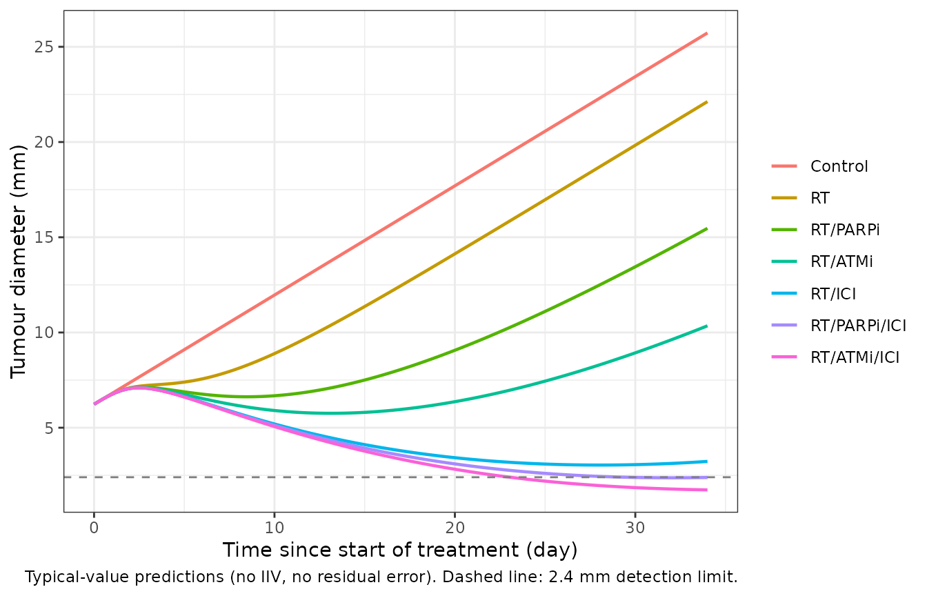
Visual predictive check against the deposited dataset
The paper’s VPC (Figure 3) simulates from Table 2 and keeps only simulated diameters of 11.44 mm or less, to mimic mice leaving the study at the tumour end point. The same rule is applied below. The points are the per-cohort medians of the deposited dataset (Data S1, 212 mice, 2143 diameters) on days 0, 7, 14 and 21; later medians rest on few surviving mice and are not shown.
# Per-cohort median tumour diameter (mm) and number of diameters, computed by
# the maintainers from Data S1 (columns ID, TIME, TRT, DV, STUDY; TRT 1 control,
# 2 RT, 3 RT/PARPi, 4.5 RT/ATMi, 5.5 RT/ICI, 6 RT/PARPi/ICI, 7 RT/ATMi/ICI).
data_s1 <- tibble::tribble(
  ~cohort,        ~time, ~median_obs, ~n_obs,
  "Control",       0,     6.170,      57,
  "Control",       7,    10.300,      50,
  "RT",            0,     6.190,      36,
  "RT",            7,     7.850,      32,
  "RT",           14,     9.930,      24,
  "RT",           21,    11.750,       8,
  "RT/PARPi",      0,     6.305,      24,
  "RT/PARPi",      7,     7.075,      24,
  "RT/PARPi",     14,     6.710,      21,
  "RT/PARPi",     21,     7.410,      14,
  "RT/ATMi",       0,     6.300,      17,
  "RT/ATMi",       7,     6.440,      14,
  "RT/ATMi",      14,     5.300,      12,
  "RT/ATMi",      21,     6.100,      10,
  "RT/ICI",        0,     6.115,      42,
  "RT/ICI",        7,     6.230,      40,
  "RT/ICI",       14,     4.970,      38,
  "RT/ICI",       21,     4.730,      30,
  "RT/PARPi/ICI",  0,     5.985,      24,
  "RT/PARPi/ICI",  7,     6.145,      22,
  "RT/PARPi/ICI", 14,     4.425,      20,
  "RT/PARPi/ICI", 21,     3.495,      18,
  "RT/ATMi/ICI",   0,     5.555,      12,
  "RT/ATMi/ICI",   7,     7.070,       9,
  "RT/ATMi/ICI",  14,     4.830,       9,
  "RT/ATMi/ICI",  21,     4.490,       9
) |>
  mutate(cohort = factor(cohort, levels = levels(cohorts$cohort)))
rxode2::rxSetSeed(20230918)
sim_vpc <- rxode2::rxSolve(mod, events, keep = "cohort", returnType = "data.frame")

vpc_summary <- function(sim) {
  sim |>
    filter(sim <= 11.44) |>
    group_by(cohort, time) |>
    summarise(
      p05 = quantile(sim, 0.05), p50 = median(sim), p95 = quantile(sim, 0.95),
      n_sim = n(), .groups = "drop"
    ) |>
    filter(n_sim >= 20)
}
vpc_rt2 <- vpc_summary(sim_vpc)

ggplot(vpc_rt2, aes(time)) +
  geom_ribbon(aes(ymin = p05, ymax = p95), fill = "steelblue", alpha = 0.25) +
  geom_line(aes(y = p50), colour = "steelblue4", linewidth = 0.8) +
  geom_point(data = data_s1, aes(y = median_obs), colour = "black") +
  facet_wrap(~cohort, ncol = 3) +
  coord_cartesian(xlim = c(0, 25), ylim = c(0, 12)) +
  labs(
    x = "Time since start of treatment (day)", y = "Tumour diameter (mm)",
    caption = paste(
      "Replicates Figure 3 of Hodson 2023: simulated median and 5th-95th percentiles",
      "(diameters <= 11.44 mm). Points: Data S1 medians."
    )
  ) +
  theme_bw()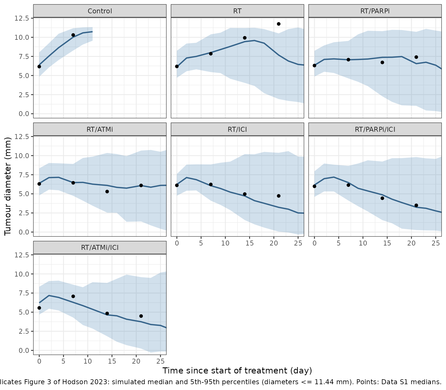
The radiotherapy window
Equation 2 prints the RT input as
R(t) = 2 Gy * Heaviside(4.1 - t), and the text describes it
as active between days 0 and 4. The NONMEM code the estimates come from
(Code S1) instead writes IF (TIME.LT.4) HEAV1 = 1 inside
$DES. In $DES, NONMEM’s TIME is
the time of the data record the integrator is advancing towards, not the
continuous time T. On the study’s measurement records (days
0, 2, 4, 7, …) the switch is therefore on while integrating from day 0
to day 2 and off from day 2 onwards: an effective 2-day RT window, half
the radiation drive of the printed equation. The packaged model defaults
to this fitted window, rt_end = 2.
The comparison below re-simulates the same cohort with
rt_end = 4 and puts the medians on days 7 and 14 (where
every cohort still has most of its mice) beside the deposited data.
rxode2::rxSetSeed(20230918)
sim_vpc4 <- rxode2::rxSolve(
  mod, events, params = c(rt_end = 4), keep = "cohort", returnType = "data.frame"
)
vpc_rt4 <- vpc_summary(sim_vpc4)

window_cmp <- data_s1 |>
  filter(time %in% c(7, 14)) |>
  left_join(select(vpc_rt2, cohort, time, sim_rt2 = p50), by = c("cohort", "time")) |>
  left_join(select(vpc_rt4, cohort, time, sim_rt4 = p50), by = c("cohort", "time"))

window_cmp |>
  select(cohort, time, median_obs, sim_rt2, sim_rt4) |>
  rename(
    Cohort = cohort, Day = time, "Data S1 median (mm)" = median_obs,
    "Simulated median, rt_end = 2 (mm)" = sim_rt2,
    "Simulated median, rt_end = 4 (mm)" = sim_rt4
  ) |>
knitr::kable(digits = 2)| Cohort | Day | Data S1 median (mm) | Simulated median, rt_end = 2 (mm) | Simulated median, rt_end = 4 (mm) |
|---|---|---|---|---|
| Control | 7 | 10.30 | 10.02 | 10.02 |
| RT | 7 | 7.85 | 8.00 | 6.45 |
| RT | 14 | 9.93 | 9.43 | 7.11 |
| RT/PARPi | 7 | 7.08 | 7.06 | 5.05 |
| RT/PARPi | 14 | 6.71 | 7.38 | 2.37 |
| RT/ATMi | 7 | 6.44 | 6.47 | 4.30 |
| RT/ATMi | 14 | 5.30 | 6.10 | 1.01 |
| RT/ICI | 7 | 6.23 | 6.07 | 3.72 |
| RT/ICI | 14 | 4.97 | 4.73 | 0.53 |
| RT/PARPi/ICI | 7 | 6.14 | 6.47 | 4.15 |
| RT/PARPi/ICI | 14 | 4.42 | 4.87 | 0.57 |
| RT/ATMi/ICI | 7 | 7.07 | 6.28 | 3.95 |
| RT/ATMi/ICI | 14 | 4.83 | 4.65 | 0.27 |
err_rt2 <- abs(window_cmp$sim_rt2 - window_cmp$median_obs)
err_rt4 <- abs(window_cmp$sim_rt4 - window_cmp$median_obs)
c(median_abs_err_rt2 = median(err_rt2, na.rm = TRUE),
  median_abs_err_rt4 = median(err_rt4, na.rm = TRUE))
#> median_abs_err_rt2 median_abs_err_rt4
#>          0.2800238          2.8223737

stopifnot(
  # The fitted window tracks the deposited medians to well under 1 mm.
  median(err_rt2, na.rm = TRUE) < 1,
  # A 4-day window shrinks the treated tumours far faster than the data.
  median(err_rt4, na.rm = TRUE) > 2
)
With rt_end = 2 the simulated medians follow the
deposited data and the paper’s Figure 3 (for example RT/ICI about 6 mm
on day 7 and 5 mm on day 14). With a 4-day window the RT/ICI tumours
have almost vanished by day 14, which neither the data nor Figure 3
show.
Simulation of alternative potencies (Figure 4)
Figure 4 explores lower anti-PD-L1 and AZD0156 potencies. Following
Methods S1, every mouse is followed to day 34; a mouse is cured if its
diameter is below the 2.4 mm detection limit on day 34, and survives if
its diameter has not reached 10 mm by day 34. Figure 4c-d report these
rates for RT/ATMi, RT/ICI and RT/ATMi/ICI at
gamma_ATMi = 4.34 and gamma_ICI = 3.9, and the
Results quote an 86% cure rate for RT/ICI at the fitted
gamma_ICI = 11.9.
These simulations reproduce the published rates only with a 4-day RT
window. The authors simulated Figure 4 on a dataset extended to have
records up to day 34 (Methods S1); with records dense enough in the
first days, the same TIME.LT.4 switch stays on for about 4
days. The chunk below therefore sets rt_end = 4.
fig4_cohorts <- tibble::tribble(
  ~cohort,                     ~TRT_RADIOTHERAPY, ~TRT_OLAPARIB, ~TRT_AZD0156, ~TRT_ANTIPDL1, ~gamma_ici,
  "RT/ATMi",                   1,                 0,             1,            0,             3.9,
  "RT/ICI",                    1,                 0,             0,            1,             3.9,
  "RT/ATMi/ICI",               1,                 0,             1,            1,             3.9,
  "RT/ICI (gamma_ICI = 11.9)", 1,                 0,             0,            1,             11.9
)
fig4_events <- bind_rows(lapply(seq_len(nrow(fig4_cohorts)), function(i) {
  make_cohort(fig4_cohorts[i, ], n_per_arm, 0:34, id_offset = (i - 1L) * n_per_arm)
})) |>
  rename(e_trt_antipdl1_kexh = gamma_ici)

rxode2::rxSetSeed(34)
sim_fig4 <- rxode2::rxSolve(
  mod, fig4_events, params = c(rt_end = 4), keep = "cohort", returnType = "data.frame"
)

fig4_rates <- sim_fig4 |>
  group_by(cohort, id) |>
  summarise(
    cured = sim[time == 34] < 2.4,
    survived = max(sim) < 10,
    .groups = "drop"
  ) |>
  group_by(cohort) |>
  summarise(cure = mean(cured), survival = mean(survived), .groups = "drop")

# Figure 4c-d bar heights (read off the figure by the maintainers) and the
# Results text (86% cure for RT/ICI at the fitted potency).
fig4_paper <- tibble::tribble(
  ~cohort,                     ~cure_paper, ~survival_paper,
  "RT/ATMi",                   0.61,        0.765,
  "RT/ICI",                    0.60,        0.752,
  "RT/ATMi/ICI",               0.785,       0.870,
  "RT/ICI (gamma_ICI = 11.9)", 0.86,        NA
)
fig4_cmp <- left_join(fig4_paper, fig4_rates, by = "cohort")
fig4_cmp |>
  select(cohort, cure_paper, cure, survival_paper, survival) |>
  rename(
    Cohort = cohort, "Cure, paper" = cure_paper, "Cure, simulated" = cure,
    "Survival, paper" = survival_paper, "Survival, simulated" = survival
  ) |>
knitr::kable(digits = 3)| Cohort | Cure, paper | Cure, simulated | Survival, paper | Survival, simulated |
|---|---|---|---|---|
| RT/ATMi | 0.610 | 0.625 | 0.765 | 0.705 |
| RT/ICI | 0.600 | 0.540 | 0.752 | 0.660 |
| RT/ATMi/ICI | 0.785 | 0.750 | 0.870 | 0.840 |
| RT/ICI (gamma_ICI = 11.9) | 0.860 | 0.880 | NA | 0.905 |
cure_err <- abs(fig4_cmp$cure - fig4_cmp$cure_paper)
surv_err <- abs(fig4_cmp$survival - fig4_cmp$survival_paper)
stopifnot(
  # 200 mice per arm: the Monte Carlo SE of a rate near 0.6 is about 0.035.
  mean(cure_err) < 0.08,
  max(cure_err) < 0.15,
  # Simulated survival sits a few points below the bars (see the table).
  mean(surv_err, na.rm = TRUE) < 0.10,
  # Tri-therapy cures more mice than either bi-therapy, as in Figure 4d.
  fig4_rates$cure[fig4_rates$cohort == "RT/ATMi/ICI"] >
    max(fig4_rates$cure[fig4_rates$cohort %in% c("RT/ATMi", "RT/ICI")])
)
fig4_cmp |>
  select(cohort, cure_paper, cure, survival_paper, survival) |>
  pivot_longer(-cohort, names_to = "key", values_to = "rate") |>
  mutate(
    endpoint = ifelse(grepl("^cure", key), "Cure at day 34", "Survival at day 34"),
    source = ifelse(grepl("_paper$", key), "Hodson 2023 Figure 4", "Simulated")
  ) |>
  filter(!is.na(rate)) |>
  ggplot(aes(cohort, rate, fill = source)) +
  geom_col(position = position_dodge(width = 0.8), width = 0.7) +
  facet_wrap(~endpoint) +
  scale_y_continuous(limits = c(0, 1)) +
  labs(
    x = NULL, y = "Fraction of mice", fill = NULL,
    caption = "Replicates Figure 4c-d of Hodson 2023 (gamma_ATMi 4.34, gamma_ICI 3.9; rt_end = 4)."
  ) +
  theme_bw() +
  theme(axis.text.x = element_text(angle = 20, hjust = 1), legend.position = "bottom")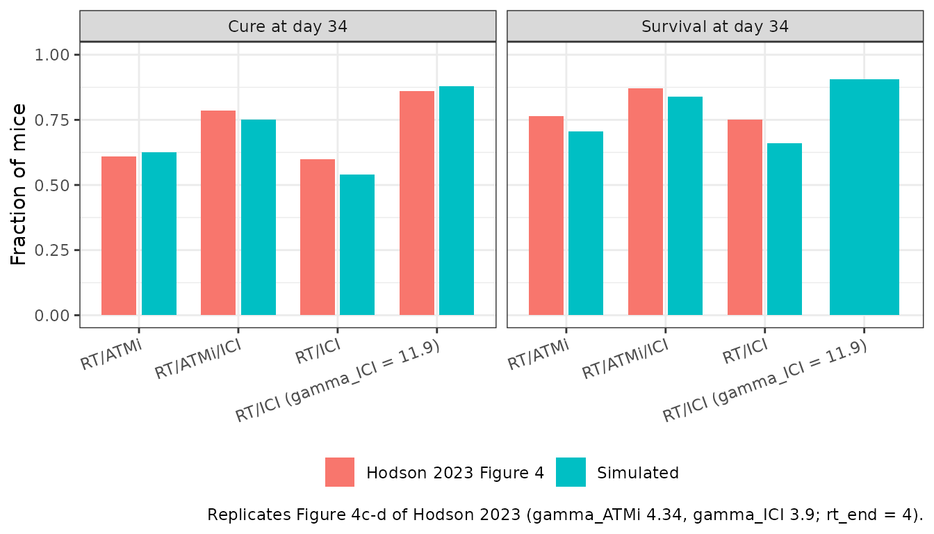
With the fitted 2-day window the same simulation cures far fewer mice: day-34 cure depends strongly on how much RT drive the model receives, which is why the window matters for anyone reusing the model.
rxode2::rxSetSeed(34)
sim_fig4_rt2 <- rxode2::rxSolve(mod, fig4_events, keep = "cohort", returnType = "data.frame")
sim_fig4_rt2 |>
  group_by(cohort, id) |>
  summarise(cured = sim[time == 34] < 2.4, .groups = "drop") |>
  group_by(cohort) |>
  summarise("Cure at day 34, rt_end = 2" = mean(cured)) |>
  rename(Cohort = cohort) |>
knitr::kable(digits = 3)| Cohort | Cure at day 34, rt_end = 2 |
|---|---|
| RT/ATMi | 0.130 |
| RT/ATMi/ICI | 0.260 |
| RT/ICI | 0.140 |
| RT/ICI (gamma_ICI = 11.9) | 0.345 |
Non-compartmental analysis
No drug concentrations are modelled: the three drugs enter as treatment indicators acting on the T-cell exhaustion rate, and RT as a fixed input. NCA with PKNCA therefore does not apply. The model is checked instead against the derived quantities of the Results, the closed-form untreated growth, the deposited dataset and the Figure 4 simulations above.
Assumptions and deviations
-
Radiotherapy window. The packaged default is
rt_end = 2days, the effective window of the published NONMEM code on the study’s Monday / Wednesday / Friday records, under which Table 2 was estimated. It reproduces the Figure 3 VPC and the deposited Data S1 medians. Equation 2 prints a 4.1-day window and Figure 4 was simulated with an effectively 4-day window; setrt_endto 4 (or 4.1) to reproduce Figure 4. No single window reproduces both figures, so the paper is internally inconsistent on this point. The maintainers chose the fitted window as the default. -
Indicator encoding. The NONMEM code derives the
flags
RT1,PARP,ATM1andIO1from a cohort codeTRT. They are carried here as the canonical indicatorsTRT_RADIOTHERAPY,TRT_OLAPARIB,TRT_AZD0156andTRT_ANTIPDL1. The model was fitted only to cohorts receiving RT (plus the untreated control), so predictions for a DDRi or ICI without RT (theTRT_RADIOTHERAPY = 0combinations) are extrapolations: without RT the model has almost no T cells for the drugs to act on. -
Residual error. Table 2’s ‘Additive RV’ of 0.506
mm^2 is the NONMEM
$SIGMAvariance; the packagedaddSdis its square root, 0.711 mm. The Results confirm the unit (‘RV is estimated to be ~0.5 mm2’). -
IIV correlations. Table 2 reports the block as
variances and correlations; the packaged covariances are written as
cor * sqrt(var_i * var_j)with the Table 2 values. - Dropout. The model has no dropout process. The VPC follows the paper in discarding simulated diameters above 11.44 mm.
- Figure 4 values are bar heights read off Figure 4c-d by the maintainers, apart from the 86% RT/ICI cure rate, which is quoted in the Results.
- Data S1 is the dataset deposited with the article for use with Code S1; its per-cohort medians were computed by the maintainers.