Eteplirsen (Patel 2025)
Source:vignettes/articles/Patel_2025_eteplirsen.Rmd
Patel_2025_eteplirsen.RmdModel and source
Citation: Patel Y, Orogun L, Yocum N, Rodino-Klapac LR, East L. A Population Pharmacokinetic Model to Inform Extension of the Eteplirsen Dosing Regimen Across the Broad DMD Population. CPT Pharmacometrics Syst Pharmacol. 2025;14(5):891-903. doi:10.1002/psp4.70001.
Description: Three-compartment IV-infusion population PK model for eteplirsen, an exon-51-skipping phosphorodiamidate morpholino oligomer (PMO), in 157 male patients with Duchenne muscular dystrophy aged 6 months to 16.4 years pooled from six clinical studies (Patel 2025). Clearance uses an age-cutoff structure at 4 years: a separate typical clearance is estimated in each age stratum (6.98 L/h for age > 4 years, 4.97 L/h for age <= 4 years), both normalized to a 37 kg reference weight and an eGFR of 145 mL/min/1.73 m^2. Body weight enters every disposition parameter allometrically with exponents fixed at 0.75 on the three clearance terms and 1 on the three volumes; cystatin-C-based CKD-EPI eGFR enters CL as a power effect with an estimated exponent of 1.60. Interindividual variability is a full 4x4 block on CL, V1, V2 and Q2 (none on V3 or Q3), and residual error is additive on the log scale. Both age strata come from a single joint NONMEM fit.
Article: https://doi.org/10.1002/psp4.70001
Supplement (Method S1, Figures S1-S6, Tables S1-S2): Data S1 of the Supporting Information, retrieved as
PSP4-14-891-s001.pdf. Table S1 (ethnicity, race and exon-deletion mutations) and Table S2 (simulated steady-state exposures and the weight-by-age distribution) are both used below.
Eteplirsen is a phosphorodiamidate morpholino oligomer (PMO) approved by the US FDA for patients with Duchenne muscular dystrophy (DMD) carrying a mutation amenable to exon 51 skipping. Patel 2025 is the first published population PK analysis for the antisense-oligonucleotide class in DMD. It pools six clinical studies to characterise disposition across the full target age range and to support extension of the uniform 30 mg/kg weekly dosing regimen to patients as young as 6 months.
Population
The analysis dataset held 3258 quantifiable eteplirsen plasma concentrations from 157 male patients with exon-51-skip-amenable DMD, pooled from six studies (Patel 2025 Table 1): NCT03218995 (4658-102, ages 6-48 months), NCT01396239 (4658-201), NCT01540409 (4658-202), NCT02420379 (4658-203), NCT00844597 (4658-28) and NCT02255552 (4658-301). Median age was 8.37 years (range 0.55 to 16.4), median body weight 27.1 kg (range 6.80 to 68.9) and median eGFR 145 mL/min/1.73 m^2 (range 85.5 to 180). All patients are male because DMD is X-linked recessive. Race was 84% White, 6% Asian, 2% Black or African American, 1% Pacific Islander, 3% Other and 4% missing; 8% were Hispanic or Latino (Table S1). Doses ranged from 0.5 to 50 mg/kg weekly as an approximately 1-hour IV infusion; 37 samples (1.1%) below the limit of quantification were excluded.
Because creatinine is a by-product of the muscle breakdown that characterises DMD, creatinine clearance is not a valid renal marker in this population. The authors therefore estimated eGFR from serum cystatin C using the CKD-EPI equation (Methods section 2.3). No subject had an eGFR below 85.5 mL/min/1.73 m^2, so the model carries no information about renal impairment.
The same information is available programmatically via the model’s
population metadata:
str(readModelDb("Patel_2025_eteplirsen")()$population, max.level = 1)
#> List of 15
#>  $ species       : chr "human"
#>  $ n_subjects    : num 157
#>  $ n_studies     : num 6
#>  $ n_observations: num 3258
#>  $ age_range     : chr "0.55-16.4 years (6 months to 16.4 years)"
#>  $ age_median    : chr "8.37 years"
#>  $ weight_range  : chr "6.80-68.9 kg"
#>  $ weight_median : chr "27.1 kg"
#>  $ sex_female_pct: num 0
#>  $ race_ethnicity: Named num [1:6] 84 2 6 1 3 4
#>   ..- attr(*, "names")= chr [1:6] "White" "Black" "Asian" "Pacific Islander" ...
#>  $ disease_state : chr "Duchenne muscular dystrophy with a confirmed mutation amenable to exon 51 skipping"
#>  $ renal_function: chr "eGFR (cystatin-C CKD-EPI) median 145 mL/min/1.73 m^2, range 85.5-180; no subject below 85.5, so the model is no"| __truncated__
#>  $ dose_range    : chr "0.5-50 mg/kg weekly as an approximately 1-h IV infusion; 30 mg/kg/week is the approved regimen"
#>  $ regions       : chr "Not reported by region; the six studies are NCT03218995 (4658-102), NCT01396239 (4658-201), NCT01540409 (4658-2"| __truncated__
#>  $ notes         : chr "Patel 2025 Table 1 (study design, N, age, weight and eGFR by study) and Table S1 (ethnicity, race and exon-dele"| __truncated__
Source trace
Every ini() entry in
inst/modeldb/specificDrugs/Patel_2025_eteplirsen.R carries
an in-file comment naming its source location. They are collected here
for review.
| Equation / parameter | Value | Source location |
|---|---|---|
lcl_agegt4 (CL, age > 4 y) |
6.98 L/h | Table 2, theta1 (95% CI 6.68-7.31) |
lcl_agele4 (CL, age <= 4 y) |
4.97 L/h | Table 2, theta2 (95% CI 4.48-5.47) |
lvc (V1) |
2.21 L | Table 2, theta3 (95% CI 1.93-2.55) |
lvp (V2) |
2.23 L | Table 2, theta4 (95% CI 1.90-2.64) |
lq (Q2) |
0.334 L/h | Table 2, theta5 (95% CI 0.262-0.422) |
lvp2 (V3) |
4.12 L | Table 2, theta6 (95% CI 3.81-4.43) |
lq2 (Q3) |
3.49 L/h | Table 2, theta7 (95% CI 3.29-3.70) |
e_crcl_cl (eGFR on CL) |
1.60 | Table 2, theta8 (95% CI 1.33-1.92) |
e_wt_cl, e_wt_q, e_wt_q2
|
0.75 (fixed) | Eq. 1, 4, 6; Results 3.3 |
e_wt_vc, e_wt_vp,
e_wt_vp2
|
1 (fixed) | Eq. 2, 3, 5; Results 3.3 |
| Reference weight | 37 kg | Results 3.4 narrative |
| Reference eGFR | 145 mL/min/1.73 m^2 | Results 3.4 narrative; Table 1 median |
| Age cutoff | 4 years | Eq. 1 ifelse(Age > 4 yrs, theta1, theta2)
|
etalcl variance |
0.05375 = log(1 + 0.235^2) | Table 2 omega_CL 23.5 CV%; Methods 2.5.1 %CV formula |
etalvc variance |
0.22154 = log(1 + 0.498^2) | Table 2 omega_V1 49.8 CV% |
etalvp variance |
0.40348 = log(1 + 0.705^2) | Table 2 omega_V2 70.5 CV% |
etalq variance |
0.72314 = log(1 + 1.030^2) | Table 2 omega_Q2 103 CV% |
| IIV covariances | 0.0541, 0.110, 0.167, 0.193, 0.295, 0.470 | Table 2 Cov() rows |
expSd |
0.34086 = sqrt(log(1 + 0.351^2)) | Table 2 sigma_RV 35.1 CV%; Methods 2.5.1 |
| Structure: 3 compartments, linear elimination | n/a | Results 3.3; Eq. 1-6 |
| Zero-order input (1-h IV infusion) | n/a | Methods 2.2; Results 3.3 |
| Residual error additive on log domain | n/a | Methods 2.5.1 |
The two clearance thetas are the only stratum-specific parameters. Everything else – volumes, inter-compartmental clearances, the eGFR exponent, the whole 4x4 IIV block and the residual error – is shared between the two age strata in a single joint NONMEM fit, so the model is one file rather than two.
Table 2 reports the structural thetas already back-transformed (its
Units column reads L/h and L) while Methods section 2.5.1 states that
parameters were “modeled in the log-domain” with
P_i = exp(P_hat + eta_Pi). Each ini() entry is
therefore written log(<Table 2 estimate>). The same
section prints the transform used for the variance terms,
%CV = 100 * sqrt(exp(omega^2) - 1), which is what fixes the
diagonal of the IIV block as log(1 + CV^2) rather than
CV^2. The resulting 4x4 matrix is positive definite
(smallest eigenvalue 0.0119, correlations 0.50 to 0.87).
Virtual cohort
Original observed data are not publicly available. The simulations below use virtual populations whose covariate distributions approximate the published demographics. Body weights are drawn from log-normal distributions matched to the median and 5th/95th percentiles of Table S2, which lists the weight distribution the authors used for their own stochastic simulation. Age is drawn uniformly within each age band and enters the model only through the 4-year cutoff. eGFR is held at the reference value of 145 mL/min/1.73 m^2 – the paper reports the weight-by-age sources for its virtual population but does not state how eGFR was simulated (see Assumptions).
set.seed(20250203)

N_PER_ARM <- 200L

age_groups <- tibble::tribble(
  ~agegrp,       ~age_lo, ~age_hi, ~wt_med, ~wt_lo, ~wt_hi,
  "0.5 to <2 y",     0.5,     2.0,    10.2,   8.19,   13.7,
  "2 to <4 y",       2.0,     4.0,    14.6,   11.3,   18.2,
  "4 to <7 y",       4.0,     7.0,    19.6,   14.7,   27.9,
  "7 to <=16 y",     7.0,    16.0,    38.1,   22.3,   74.3
)

# Dense sampling over the first day (where all the structure is) and a coarse
# tail out to the end of the 168 h dosing interval.
OBS_TIMES <- c(seq(0, 24, by = 0.1), seq(26, 168, by = 2))

make_cohort <- function(n, age_lo, age_hi, wt_med, wt_lo, wt_hi, label,
                        mgkg = 30, crcl = 145, id_offset = 0L,
                        obs_times = OBS_TIMES) {
  sdlog <- (log(wt_hi) - log(wt_lo)) / (2 * stats::qnorm(0.95))
  subj <- tibble::tibble(
    id    = id_offset + seq_len(n),
    AGE   = stats::runif(n, age_lo, age_hi),
    WT    = stats::rlnorm(n, log(wt_med), sdlog),
    CRCL  = crcl,
    mgkg  = mgkg,
    agegrp = label
  )
  doses <- subj |>
    dplyr::mutate(
      time = 0, evid = 1L, cmt = "central",
      amt  = mgkg * WT,
      # rate = amt / 1 h reproduces the approximately 1-hour IV infusion of
      # Methods section 2.2 (the "zero-order absorption" of Results 3.3).
      rate = mgkg * WT
    )
  obs <- tidyr::expand_grid(subj, time = obs_times) |>
    dplyr::mutate(evid = 0L, cmt = "central", amt = NA_real_, rate = NA_real_)
  dplyr::bind_rows(doses, obs) |>
    dplyr::arrange(id, time, dplyr::desc(evid))
}

events <- dplyr::bind_rows(
  lapply(seq_len(nrow(age_groups)), function(i) {
    g <- age_groups[i, ]
    make_cohort(
      n = N_PER_ARM, age_lo = g$age_lo, age_hi = g$age_hi,
      wt_med = g$wt_med, wt_lo = g$wt_lo, wt_hi = g$wt_hi,
      label = g$agegrp, id_offset = (i - 1L) * N_PER_ARM
    )
  })
)

# Disjoint IDs across cohorts are mandatory: duplicate IDs silently merge into
# one subject that receives the summed dose.
stopifnot(!anyDuplicated(unique(events[, c("id", "time", "evid")])))
stopifnot(dplyr::n_distinct(events$id) == N_PER_ARM * nrow(age_groups))
Simulation
mod <- readModelDb("Patel_2025_eteplirsen")

sim <- rxode2::rxSolve(
  mod, events = events,
  keep = c("agegrp", "WT", "AGE", "CRCL", "mgkg"),
  # The 168 h tail of a weekly interval sits at 1e-7 to 1e-14 of Cmax. At the
  # default tolerances the ODE integrator undershoots zero there (observed:
  # -1.5e-8 ug/mL in 9 of 800 subjects); tight tolerances shrink that to the
  # 1e-12 level. The NCA below additionally drops the numerically-zero tail.
  rtol = 1e-10, atol = 1e-12
) |>
  as.data.frame()

# rxSolve can silently drop subjects; assert the count survived.
stopifnot(dplyr::n_distinct(sim$id) == N_PER_ARM * nrow(age_groups))
Weekly dosing with a short half-life produces essentially no accumulation, which is why Patel 2025 could assume steady state at the first simulated dose (Methods section 2.8). The check below confirms that concentration at the end of the 168 h dosing interval is a negligible fraction of Cmax, so a single-dose profile over 0-168 h is the steady-state dosing interval.
sim |>
  dplyr::group_by(id) |>
  dplyr::summarise(
    cmax  = max(Cc),
    ctau  = Cc[which.max(time)],
    .groups = "drop"
  ) |>
  dplyr::summarise(
    `Max C(168 h) / Cmax across subjects` = format(max(ctau / cmax), scientific = TRUE, digits = 3),
    `Median C(168 h) / Cmax`              = format(stats::median(ctau / cmax), scientific = TRUE, digits = 3)
  ) |>
knitr::kable(caption = "Accumulation check: residual concentration at the end of the weekly dosing interval, relative to Cmax.")| Max C(168 h) / Cmax across subjects | Median C(168 h) / Cmax |
|---|---|
| 4.87e-07 | 1.07e-14 |
Replicate published figures
Figure 1 – dose-normalised concentrations superimpose across dose levels
Patel 2025 Figure 1 plots dose-normalised eteplirsen concentration versus time coloured by dose group and reports that the profiles “were superimposed without evidence of any clear trends”, supporting linear PK across 0.5-50 mg/kg. The model is linear by construction, so this is a check that the packaged implementation carries no dose-dependent term.
dose_levels <- c(0.5, 2, 10, 30, 50)

events_dose <- dplyr::bind_rows(
  lapply(seq_along(dose_levels), function(i) {
    make_cohort(
      n = 50L, age_lo = 0.55, age_hi = 16.4,
      wt_med = 27.1, wt_lo = 8.0, wt_hi = 62.0,
      label = paste0(dose_levels[i], " mg/kg"),
      mgkg = dose_levels[i], id_offset = (i - 1L) * 50L,
      obs_times = seq(0, 24, by = 0.25)
    )
  })
)
stopifnot(!anyDuplicated(unique(events_dose[, c("id", "time", "evid")])))

sim_dose <- rxode2::rxSolve(
  mod, events = events_dose, keep = c("agegrp", "WT", "mgkg")
) |>
  as.data.frame() |>
  dplyr::rename(dose_group = agegrp)

sim_dose |>
  dplyr::filter(Cc > 0) |>
  dplyr::mutate(cc_norm = Cc / mgkg) |>
  dplyr::group_by(dose_group, time) |>
  dplyr::summarise(Q50 = stats::median(cc_norm), .groups = "drop") |>
  ggplot(aes(time, Q50, colour = dose_group)) +
  geom_line(linewidth = 0.8) +
  scale_y_log10() +
  labs(
    x = "Time after start of infusion (h)",
    y = "Dose-normalised Cc (ug/mL per mg/kg)",
    colour = "Dose group",
    title = "Figure 1 -- dose-normalised concentration-time profiles",
    caption = "Replicates Figure 1 of Patel 2025."
  )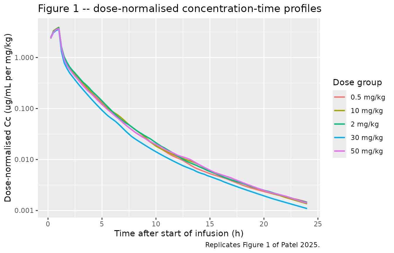
Figure 3 – concentration versus time after dose
Patel 2025 Figure 3a is a prediction-corrected VPC of eteplirsen concentration versus time after dose. The panel below shows the simulated median with the 5th-95th prediction interval over the first 24 h, the window the paper’s own simulation used.
sim |>
  dplyr::filter(time > 0, time <= 24, Cc > 0) |>
  dplyr::group_by(time) |>
  dplyr::summarise(
    Q05 = stats::quantile(Cc, 0.05),
    Q50 = stats::median(Cc),
    Q95 = stats::quantile(Cc, 0.95),
    .groups = "drop"
  ) |>
  ggplot(aes(time, Q50)) +
  geom_ribbon(aes(ymin = Q05, ymax = Q95), alpha = 0.25) +
  geom_line(linewidth = 0.8) +
  scale_y_log10() +
  labs(
    x = "Time after start of infusion (h)", y = "Cc (ug/mL)",
    title = "Figure 3 -- simulated median and 5th-95th prediction interval",
    caption = "Replicates the shape of Figure 3a of Patel 2025 (30 mg/kg weekly, all age groups pooled)."
  )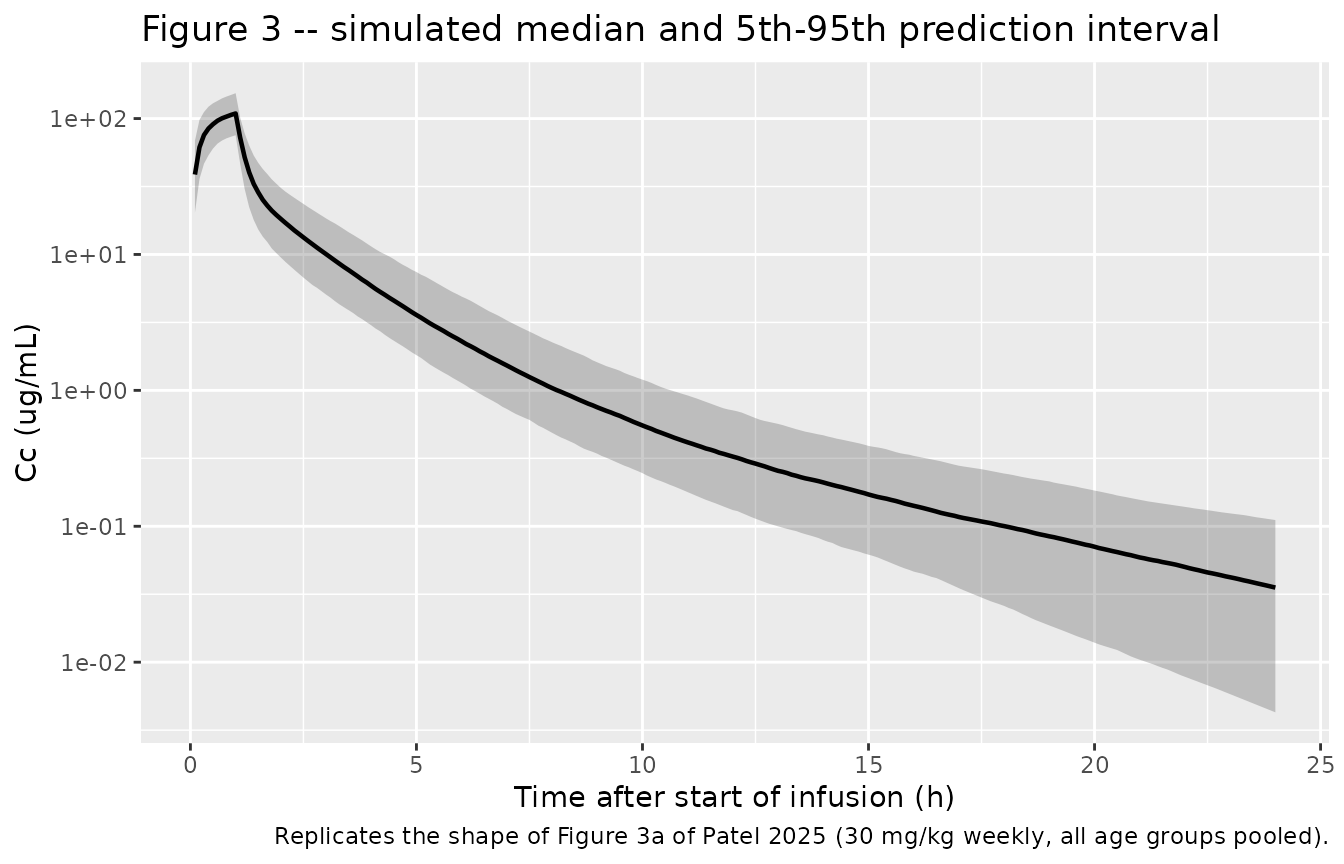
The profile shows the features the paper describes in Results section 3.2: concentration peaks at the end of the 1-hour infusion, a rapid distribution phase follows over the next 2-3 h, and a slower elimination phase runs out over the remainder of the day.
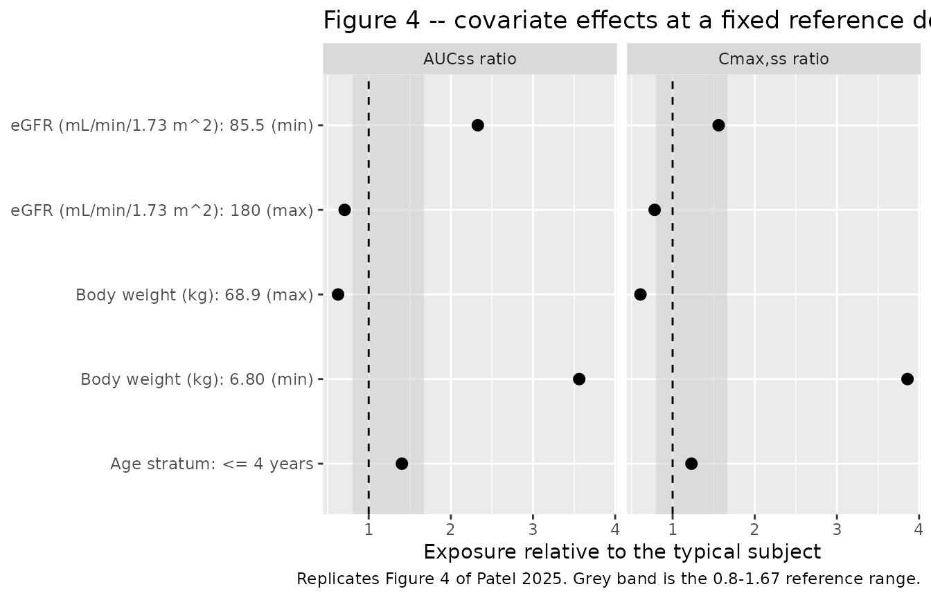
Figure 4 – covariate effects on normalised steady-state exposure
Figure 4 of Patel 2025 is a forest plot of steady-state AUC and Cmax relative to a typical subject, evaluated at a reference dose (so the body-weight effect is not cancelled by weight-based dosing), against a reference range of 0.8-1.67. The reference subject is a patient older than 4 years weighing 37 kg with an eGFR of 145 mL/min/1.73 m^2.
mod_typical <- rxode2::zeroRe(mod)

REF_DOSE <- 30 * 37  # mg, the 30 mg/kg dose of the 37 kg reference patient

typical_exposure <- function(wt = 37, crcl = 145, age = 8) {
  ev <- tibble::tibble(
    id = 1L, time = c(0, seq(0, 168, by = 0.05)),
    evid = c(1L, rep(0L, length(seq(0, 168, by = 0.05)))),
    cmt = "central",
    amt = c(REF_DOSE, rep(NA_real_, length(seq(0, 168, by = 0.05)))),
    rate = c(REF_DOSE, rep(NA_real_, length(seq(0, 168, by = 0.05)))),
    WT = wt, CRCL = crcl, AGE = age
  ) |>
    dplyr::arrange(time, dplyr::desc(evid))
  s <- rxode2::rxSolve(mod_typical, events = ev) |> as.data.frame()
  s <- s[order(s$time), ]
  c(
    cmax = max(s$Cc),
    auc  = sum(diff(s$time) * (utils::head(s$Cc, -1) + utils::tail(s$Cc, -1)) / 2)
  )
}

ref <- typical_exposure()
#> ℹ omega/sigma items treated as zero: 'etalcl', 'etalvc', 'etalvp', 'etalq'

forest <- dplyr::bind_rows(
  tibble::tibble(
    covariate = "Body weight (kg)",
    level     = c("6.80 (min)", "68.9 (max)"),
    value     = c(6.80, 68.9)
  ) |>
    dplyr::rowwise() |>
    dplyr::mutate(e = list(typical_exposure(wt = value))) |>
    dplyr::ungroup(),
  tibble::tibble(
    covariate = "eGFR (mL/min/1.73 m^2)",
    level     = c("85.5 (min)", "180 (max)"),
    value     = c(85.5, 180)
  ) |>
    dplyr::rowwise() |>
    dplyr::mutate(e = list(typical_exposure(crcl = value))) |>
    dplyr::ungroup(),
  tibble::tibble(
    covariate = "Age stratum",
    level     = "<= 4 years",
    value     = 2
  ) |>
    dplyr::rowwise() |>
    dplyr::mutate(e = list(typical_exposure(age = value))) |>
    dplyr::ungroup()
) |>
  dplyr::mutate(
    `AUCss ratio`   = vapply(e, function(x) unname(x["auc"]), numeric(1)) / ref[["auc"]],
    `Cmax,ss ratio` = vapply(e, function(x) unname(x["cmax"]), numeric(1)) / ref[["cmax"]]
  ) |>
  dplyr::select(-e, -value)
#> ℹ omega/sigma items treated as zero: 'etalcl', 'etalvc', 'etalvp', 'etalq'
#> ℹ omega/sigma items treated as zero: 'etalcl', 'etalvc', 'etalvp', 'etalq'
#> ℹ omega/sigma items treated as zero: 'etalcl', 'etalvc', 'etalvp', 'etalq'
#> ℹ omega/sigma items treated as zero: 'etalcl', 'etalvc', 'etalvp', 'etalq'
#> ℹ omega/sigma items treated as zero: 'etalcl', 'etalvc', 'etalvp', 'etalq'

forest |>
  tidyr::pivot_longer(c(`AUCss ratio`, `Cmax,ss ratio`),
                      names_to = "metric", values_to = "ratio") |>
  ggplot(aes(ratio, paste(covariate, level, sep = ": "))) +
  annotate("rect", xmin = 0.8, xmax = 1.67, ymin = -Inf, ymax = Inf,
           fill = "grey80", alpha = 0.5) +
  geom_vline(xintercept = 1, linetype = "dashed") +
  geom_point(size = 2.5) +
  facet_wrap(~metric) +
  labs(
    x = "Exposure relative to the typical subject", y = NULL,
    title = "Figure 4 -- covariate effects at a fixed reference dose",
    caption = "Replicates Figure 4 of Patel 2025. Grey band is the 0.8-1.67 reference range."
  )
forest |>
  knitr::kable(
    digits = 3,
    caption = "Normalised steady-state exposure by covariate level, at a fixed 1110 mg dose."
)| covariate | level | AUCss ratio | Cmax,ss ratio |
|---|---|---|---|
| Body weight (kg) | 6.80 (min) | 3.563 | 3.859 |
| Body weight (kg) | 68.9 (max) | 0.627 | 0.608 |
| eGFR (mL/min/1.73 m^2) | 85.5 (min) | 2.328 | 1.560 |
| eGFR (mL/min/1.73 m^2) | 180 (max) | 0.708 | 0.781 |
| Age stratum | <= 4 years | 1.404 | 1.229 |
This reproduces the paper’s three qualitative conclusions (Results section 3.5):
- Body weight is the only significant covariate. Both the minimum and the maximum observed weight put the point estimate outside the 0.8-1.67 band, for both AUC and Cmax.
- Age <= 4 years is not significant. The AUC ratio is 1.4, inside the band. Propagating the published 95% CIs of the two clearance thetas gives a worst case of 7.31 / 4.48 = 1.63, still inside the band – matching the paper’s statement that “the point estimate and 95% CI for the exposure parameters were within reference range”.
-
eGFR is retained but not significant. Note that the
min/max eGFR values used above do fall outside the band,
whereas the paper reports the low-eGFR effect as non-significant and the
high-eGFR effect only as “inconclusive”. With the point estimate of
1.60, the fixed-dose exposure ratio
(eGFR/145)^-1.60crosses the upper bound of 1.67 at eGFR = 105 and the lower bound of 0.8 at eGFR = 167. Both crossing points lie inside the observed 85.5-180 range, so Figure 4 of the paper must have used a narrower covariate range than the Table 1 min-max – most likely observed percentiles. The paper does not report which values Figure 4 used, so this is noted rather than reconstructed.
Figure 5 and Table S2 – steady-state exposure by age group
exposure <- sim |>
  dplyr::group_by(agegrp, id) |>
  dplyr::arrange(time, .by_group = TRUE) |>
  dplyr::summarise(
    `Cmax,ss (ug/mL)`  = max(Cc),
    `AUCss (ug*h/mL)`  = sum(diff(time) * (utils::head(Cc, -1) + utils::tail(Cc, -1)) / 2),
    .groups = "drop"
  ) |>
  dplyr::mutate(agegrp = factor(agegrp, levels = age_groups$agegrp))

exposure |>
  tidyr::pivot_longer(c(`Cmax,ss (ug/mL)`, `AUCss (ug*h/mL)`),
                      names_to = "metric", values_to = "value") |>
  ggplot(aes(agegrp, value)) +
  geom_boxplot(outlier.size = 0.6) +
  facet_wrap(~metric, scales = "free_y") +
  labs(
    x = "Age group", y = NULL,
    title = "Figure 5 -- steady-state exposure at 30 mg/kg weekly by age group",
    caption = "Replicates Figure 5 of Patel 2025."
  ) +
  theme(axis.text.x = element_text(angle = 20, hjust = 1))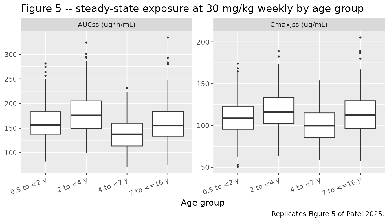
Structural identity: AUCss x CL = Dose, per subject
For any linear model the steady-state exposure over a full dosing
interval satisfies AUCss = Dose / CL exactly.
rxSolve returns each subject’s individual clearance, so
this identity can be asserted per subject rather than compared as a
median – a much sharper test, and the one that pins down where the Table
S2 discrepancy discussed below actually lives.
identity_check <- sim |>
  dplyr::group_by(id, agegrp) |>
  dplyr::arrange(time, .by_group = TRUE) |>
  dplyr::summarise(
    cl    = dplyr::first(cl),
    WT    = dplyr::first(WT),
    auc   = sum(diff(time) * (utils::head(Cc, -1) + utils::tail(Cc, -1)) / 2),
    .groups = "drop"
  ) |>
  dplyr::mutate(
    dose     = 30 * WT,
    implied  = auc * cl,
    rel_err  = implied / dose - 1
  )

# Trapezoidal error on the coarse post-24 h grid is the only source of
# deviation; assert it is under 1% for every single subject.
stopifnot(max(abs(identity_check$rel_err)) < 0.01)

tibble::tibble(
  `Max |AUC * CL / Dose - 1| across all 800 subjects` =
    sprintf("%.4f%%", 100 * max(abs(identity_check$rel_err)))
) |>
knitr::kable(caption = "Per-subject structural identity AUCss x CL = Dose.")| Max |AUC * CL / Dose - 1| across all 800 subjects |
|---|
| 0.0068% |
Because the identity holds to four decimal places for every subject, any mismatch against a published AUCss value is a statement about the published clearance, not about the simulation.
PKNCA validation
NCA is computed with PKNCA over the full 168 h steady-state dosing interval, grouped by age band so the results line up with Table S2.
sim_nca <- sim |>
  dplyr::filter(!is.na(Cc)) |>
  dplyr::select(id, time, Cc, agegrp)

# Drop the numerically-zero tail before NCA. Beyond ~1e-6 of Cmax the ODE
# integrator's absolute error is comparable to the true concentration, and a
# single undershoot below zero there turns PKNCA's log-down trapezoid into a
# NaN AUC (observed for 9 of 800 subjects at the default tolerances). Keep each
# subject's profile up to the last point at or above 1e-6 of its peak; the
# discarded tail holds < 1e-6 of the AUC.
sim_nca <- sim_nca |>
  dplyr::group_by(id) |>
  dplyr::filter(time <= max(time[Cc >= 1e-6 * max(Cc)])) |>
  dplyr::ungroup()

# Guarantee a time-zero record per subject (pre-infusion Cc is 0 for an IV
# infusion). Without it PKNCA warns "Requesting an AUC range starting (0)
# before the first measurement" once per subject.
sim_nca <- dplyr::bind_rows(
  sim_nca,
  sim_nca |> dplyr::distinct(id, agegrp) |> dplyr::mutate(time = 0, Cc = 0)
) |>
  dplyr::distinct(id, agegrp, time, .keep_all = TRUE) |>
  dplyr::arrange(id, time)

dose_df <- events |>
  dplyr::filter(evid == 1L) |>
  dplyr::select(id, time, amt, agegrp)

conc_obj <- PKNCA::PKNCAconc(
  sim_nca, Cc ~ time | agegrp + id,
  concu = "ug/mL", timeu = "h"
)
dose_obj <- PKNCA::PKNCAdose(
  dose_df, amt ~ time | agegrp + id,
  doseu = "mg"
)

intervals <- data.frame(
  start    = 0,
  end      = 168,
  cmax     = TRUE,
  tmax     = TRUE,
  auclast  = TRUE,
  cav      = TRUE,
  half.life = TRUE
)

nca_res <- PKNCA::pk.nca(
  PKNCA::PKNCAdata(conc_obj, dose_obj, intervals = intervals)
)
as.data.frame(nca_res) |>
  dplyr::filter(PPTESTCD %in% c("cmax", "tmax", "auclast", "half.life")) |>
  dplyr::group_by(agegrp, PPTESTCD) |>
  dplyr::summarise(
    median = stats::median(PPORRES),
    p2.5   = stats::quantile(PPORRES, 0.025),
    p97.5  = stats::quantile(PPORRES, 0.975),
    .groups = "drop"
  ) |>
  dplyr::mutate(agegrp = factor(agegrp, levels = age_groups$agegrp)) |>
  dplyr::arrange(agegrp, PPTESTCD) |>
  dplyr::rename(
    "Age group"  = agegrp,
    "Parameter"  = PPTESTCD,
    "Median"     = median,
    "2.5th pctl" = p2.5,
    "97.5th pctl" = p97.5
  ) |>
knitr::kable(digits = 2, caption = "Simulated steady-state NCA by age group (n = 200 per group).")| Age group | Parameter | Median | 2.5th pctl | 97.5th pctl |
|---|---|---|---|---|
| 0.5 to <2 y | auclast | 156.28 | 103.14 | 247.85 |
| 0.5 to <2 y | cmax | 108.64 | 72.12 | 160.66 |
| 0.5 to <2 y | half.life | 3.61 | 1.76 | 6.87 |
| 0.5 to <2 y | tmax | 1.00 | 1.00 | 1.00 |
| 2 to <4 y | auclast | 175.65 | 111.73 | 279.04 |
| 2 to <4 y | cmax | 116.14 | 76.46 | 167.78 |
| 2 to <4 y | half.life | 4.16 | 2.04 | 8.80 |
| 2 to <4 y | tmax | 1.00 | 1.00 | 1.00 |
| 4 to <7 y | auclast | 137.37 | 87.22 | 206.93 |
| 4 to <7 y | cmax | 99.84 | 64.58 | 146.29 |
| 4 to <7 y | half.life | 4.19 | 2.24 | 8.46 |
| 4 to <7 y | tmax | 1.00 | 1.00 | 1.00 |
| 7 to <=16 y | auclast | 155.07 | 101.36 | 245.11 |
| 7 to <=16 y | cmax | 112.22 | 70.82 | 166.83 |
| 7 to <=16 y | half.life | 4.39 | 2.29 | 10.95 |
| 7 to <=16 y | tmax | 1.00 | 1.00 | 1.00 |
Comparison against published NCA
Table S2 of Patel 2025 reports simulated steady-state AUC and Cmax by age group as median (95% CI). Those are the reference values below.
published <- tibble::tribble(
  ~agegrp,        ~cmax,  ~auclast,
  "0.5 to <2 y",  119.0,  159.0,
  "2 to <4 y",    112.0,  135.0,
  "4 to <7 y",     98.1,  106.0,
  "7 to <=16 y",  119.0,  140.0
)

cmp <- nlmixr2lib::ncaComparisonTable(
  simulated = nca_res,
  reference = published,
  by        = "agegrp",
  params    = c("cmax", "auclast"),
  units     = c(cmax = "ug/mL", auclast = "ug*h/mL"),
  tolerance_pct = 20
)

knitr::kable(
  cmp,
  caption = "Simulated vs. published steady-state exposure (Patel 2025 Table S2). * differs from reference by more than 20%."
)| NCA parameter | agegrp | Reference | Simulated | % diff |
|---|---|---|---|---|
| Cmax (ug/mL) | 0.5 to <2 y | 119 | 109 | -8.7% |
| Cmax (ug/mL) | 2 to <4 y | 112 | 116 | +3.7% |
| Cmax (ug/mL) | 4 to <7 y | 98.1 | 99.8 | +1.8% |
| Cmax (ug/mL) | 7 to <=16 y | 119 | 112 | -5.7% |
| AUClast (ug*h/mL) | 0.5 to <2 y | 159 | 156 | -1.7% |
| AUClast (ug*h/mL) | 2 to <4 y | 135 | 176 | +30.1%* |
| AUClast (ug*h/mL) | 4 to <7 y | 106 | 137 | +29.6%* |
| AUClast (ug*h/mL) | 7 to <=16 y | 140 | 155 | +10.8% |
The Cmax,ss column reproduces across all four age bands (-8.7% to +3.7%), with no row flagged. The dispersion reproduces too: the simulated 2.5th-97.5th percentile intervals in the NCA summary table above sit close to the published 95% CIs of Table S2 (for the youngest group, 80.0-167 published). Since Cmax is driven mainly by the three volumes and the infusion duration, this validates the structural model, V1/V2/V3, and the IIV block.
The AUCss column differs by -1.7% to +30.1%: it
reproduces for the youngest band alone and is over-predicted for the
other three. Given the per-subject AUCss x CL = Dose
identity asserted above, this is a statement about the published table
rather than about the implementation – see Errata below.
Assumptions and deviations
- eGFR distribution. Patel 2025 states the sources for the weight-by-age distribution of its virtual population (CDC NHANES for age < 2 years, West et al. 2013 for ages 2-12, the analysis dataset above 12) but does not say how eGFR was simulated. eGFR is therefore held at the reference value of 145 mL/min/1.73 m^2 – the cohort median from Table 1 and the normalising constant in Eq. 1 – for every simulated subject. Because the eGFR exponent is 1.60, exposure is sensitive to this choice: a 10% shift in eGFR moves AUC by about 16%.
- Age distribution. Age is drawn uniformly within each published age band. Age enters the model only through the 4-year cutoff, so only the fraction of each band above or below 4 years matters, and every band lies wholly on one side of the cutoff.
- Weight distribution. Body weight is drawn from a log-normal fitted to the median and 5th/95th percentiles reported in Table S2. The underlying distribution shape is not published.
- Steady state via a single dose. Patel 2025 assumed steady state at the first simulated dose. The accumulation check above confirms this is exact to within a negligible residual, so the vignette simulates a single dose over one 168 h dosing interval rather than a dosing series.
- Figure 4 covariate range. The covariate values used in the paper’s forest plot are not reported numerically; the min/max of Table 1 are used here, and the range that would reproduce the paper’s eGFR conclusions is reconstructed in the narrative rather than assumed.
-
No non-paper-derived parameter values. Every
ini()entry comes from Patel 2025 Table 2 or Equations 1-6. Nothing was digitised from a figure, obtained by correspondence, or carried from an upstream model, and no value was tuned to improve agreement with any published output.
Errata and unresolved discrepancies
1. Table S2 AUCss is not reproducible from Equations
1-6. For any linear model the steady-state exposure over a
dosing interval satisfies the exact identity
AUCss = Dose / CL. With a weight-based dose of 30 mg/kg and
Eq. 1, this gives
AUCss = 30 * WT / (CL_typ * (WT/37)^0.75 * (eGFR/145)^1.60)
      proportional to WT^0.25   (at fixed CL stratum and eGFR)
so within one age stratum AUCss must increase with body weight. Table S2 reports AUCss falling from 159 to 135 ug*h/mL as the median weight rises from 10.2 to 14.6 kg – both rows in the age <= 4 y stratum, where the typical clearance is the same 4.97 L/h. No value of the unreported eGFR distribution can produce that ordering together with the published allometric exponent.
Three candidate explanations were tested and all fail:
- An unreported eGFR distribution. Solving for the eGFR that would reproduce each published AUCss gives 147, 172, 169 and 158 mL/min/1.73 m^2 for the four bands. Those are implausible as age-band medians – the study cohorts closest to each band have observed median eGFR of 142 (ages 6-48 months), 149 (ages 4-6 years) and 143 (ages 7-16 years) per Table 1 – and imposing them degrades the Cmax,ss agreement into a systematic negative bias, whereas at eGFR = 145 the Cmax residuals are scattered about zero.
- A different reference weight. No single alternative reconciles the four rows: the implied reference weights are 36, 26, 27 and 31 kg.
- A 24-hour integration window. Methods section 2.8 states that simulated subjects were “followed 24 h post dose”, which raises the possibility that Table S2 reports AUC over 0-24 h rather than over the full 168 h dosing interval. It does not: at the four Table S2 median weights, typical-value AUC(0-24 h) recovers 99.8% or more of AUC(0-168 h), so the two windows are interchangeable here and the choice cannot account for a 30% gap.
The Cmax,ss column of Table S2 does agree in magnitude, which is why the discrepancy is isolated to the AUCss column: Cmax is roughly three times less sensitive to clearance than AUC is. It is worth noting, though, that the Cmax column shows the same within-stratum ordering anomaly in miniature (119 then 112 ug/mL as weight rises from 10.2 to 14.6 kg, where the model requires a slight increase); the ordering is simply small enough to stay inside the 20% tolerance. Both columns therefore point the same way.
None of this affects the packaged model, whose parameters are taken
verbatim from Table 2 and Equations 1-6 and which satisfies
AUCss = Dose / CL exactly for every simulated subject.
2. The eGFR sensitivity quoted in Results section 3.4 is internally inconsistent with Eq. 1. The paper states that raising eGFR to 160 mL/min/1.73 m^2 increases CL by 14.5% and that lowering it to 130 decreases CL by 18.4%. Applying Eq. 1 with theta8 = 1.60 and the stated reference of 145 gives +17.1% and -16.0% respectively. Both quoted percentages are consistent with a reference eGFR near 147 rather than 145; the difference is immaterial (about 1.4% in the normalising constant) and the model uses the reference of 145 that Eq. 1 and the Results 3.4 narrative both state explicitly.
3. Epsilon shrinkage is high. Table 2 notes epsilon-shrinkage of 67.7% for the residual variability, so individual-level residual diagnostics from this model should be treated with caution. Eta shrinkage is modest (11.0%, 22.1%, 24.9% and 20.4% for CL, V1, V2 and Q2).
4. Model applicability outside the observed eGFR range. No subject had an eGFR below 85.5 mL/min/1.73 m^2. The paper states explicitly that “model application below observed eGFR range would be limited”. With an exponent of 1.60 on a strongly supranormal reference of 145, extrapolation into renal impairment will over-predict the reduction in clearance.