Treosulfan (Danielak 2017)
Source:vignettes/articles/Danielak_2017_treosulfan.Rmd
Danielak_2017_treosulfan.RmdModel and source
- Citation: Danielak D, Twardosz J, Kasprzyk A, Wachowiak J, Kalwak K, Glowka F. Population pharmacokinetics of treosulfan and development of a limited sampling strategy in children prior to hematopoietic stem cell transplantation. Eur J Clin Pharmacol. 2018 Jan;74(1):79-89.
- DOI: https://doi.org/10.1007/s00228-017-2344-x
- Model description: Two-compartment IV-infusion population PK model for treosulfan (TREO) in pediatric patients undergoing conditioning prior to hematopoietic stem cell transplantation (Danielak 2017). Allometric body-weight scaling normalised to a 70 kg adult typical value with exponents fixed at 0.75 on CL and 1 on V1 and V2; Q has no weight covariate. Correlated IIV on CL and V1 (Cl-V1 correlation 0.714); independent IIV on Q. Proportional residual error.
Population
The model was developed from data collected 2007-2011 at the Department of Oncology, Hematology and Pediatric Transplantation (Poznan University of Medical Sciences) and the Department of Pediatric Hematology, Oncology and Bone Marrow Transplantation (Wroclaw Medical University). Fifteen pediatric patients (12 boys, 3 girls; age 7.8 +/- 4.9 years, range 0.4-15; body weight 26.9 +/- 15.7 kg, range 7.7-52; body surface area 0.95 +/- 0.44 m^2) received treosulfan-based conditioning prior to allogeneic hematopoietic stem cell transplantation. Diagnoses spanned hematologic malignancies (ALL 4, AML 1, CML 1), solid tumors (neuroblastoma 2, Ewing sarcoma 2), and non-malignant disorders (adrenoleukodystrophy 2, Diamond-Blackfan anemia 1, severe congenital neutropenia 1, Wiskott-Aldrich syndrome 1). Treosulfan was administered IV at 10, 12, or 14 g/m^2 once daily as a 1 h or 2 h infusion. A total of 110 plasma concentrations were collected on day 1 of therapy across two sparse-sampling protocols (6 timepoints in 7 subjects; 10 timepoints in 8 subjects); all observed concentrations were above the HPLC-MS/MS LOQ of 0.2 uM. Creatinine clearance (available for 8 of 15 patients) and sex were tested and not retained as covariates; only body weight survived backward elimination (Danielak 2017 Methods + Table 1).
The full demographics list, including age strata, dosing regimens,
and disease state breakdown, is encoded in the model file under the
population metadata block (Danielak 2017 Table 1).
Source trace
The per-parameter origin is also recorded as an in-file comment next
to each ini() entry in
inst/modeldb/specificDrugs/Danielak_2017_treosulfan.R. The
table below consolidates them.
| Equation / parameter | Value | Source location |
|---|---|---|
lcl (CL at 70 kg) |
log(14.7 L/h) | Danielak 2017 Table 2 (RSE 6.9 percent) |
lvc (V1 at 70 kg) |
log(26.0 L) | Danielak 2017 Table 2 (RSE 14.0 percent) |
lq (Q) |
log(2.25 L/h) | Danielak 2017 Table 2 (RSE 22.2 percent; no WT covariate) |
lvp (V2 at 70 kg) |
log(9.93 L) | Danielak 2017 Table 2 (RSE 9.0 percent) |
e_wt_cl |
fixed(0.75) | Danielak 2017 Table 2 (“beta Cl, weight 0.75 (fixed)”) |
e_wt_vc |
fixed(1.0) | Danielak 2017 Table 2 (“beta V1, weight 1 (fixed)”) |
e_wt_vp |
fixed(1.0) | Danielak 2017 Table 2 (“beta V2, weight 1 (fixed)”) |
var(etalcl) |
0.065025 | Danielak 2017 Table 2 (omega_Cl 25.5 percent -> 0.255^2) |
var(etalvc) |
0.264196 | Danielak 2017 Table 2 (omega_V1 51.4 percent -> 0.514^2) |
cov(etalcl, etalvc) |
0.093596 | Danielak 2017 Table 2 (rho_Cl-V1 0.714 -> rho * omega1 * omega2) |
var(etalq) |
0.148996 | Danielak 2017 Table 2 (omega_Q 38.6 percent -> 0.386^2) |
propSd |
0.188 | Danielak 2017 Table 2 (proportional residual error) |
| WT covariate equation | (WT/70)^beta |
Danielak 2017 Eq. 9 |
| Two-compartment ODE | linear IV-infusion | Danielak 2017 Methods “Structural and error model selection” |
Virtual cohort
Individual subject-level data are not publicly available. The virtual
cohort below mirrors the paper’s Table 1 demographics: weights drawn
from a log-normal centered on the cohort mean (26.9 kg) and clipped to
the observed range (7.7-52 kg). Body surface area is derived from weight
via the Costeff (1966) pediatric formula
BSA = (4*WT + 7)/(WT + 90), which gives BSA values within a
few percent of the Mosteller method used by the paper across the source
weight range. The cohort is replicated across the three dosing regimens
of the original study (12 g/m^2 over 1 h; 12 g/m^2 over 2 h; 14 g/m^2
over 2 h), so per-regimen typical-value behaviour can be compared.
set.seed(20260529)

n_per_arm <- 100L

# Weight distribution per Table 1 (mean 26.9 kg, SD 15.7 kg, range 7.7-52).
# Use a log-normal whose first two moments approximate the reported mean
# and SD on the natural scale, then truncate to the source range.
mu_wt <- 26.9
sd_wt <- 15.7
ln_sd  <- sqrt(log(1 + (sd_wt / mu_wt)^2))
ln_mu  <- log(mu_wt) - ln_sd^2 / 2

draw_weights <- function(n) {
  w <- numeric(0)
  while (length(w) < n) {
    candidate <- rlnorm(n, ln_mu, ln_sd)
    w <- c(w, candidate[candidate >= 7.7 & candidate <= 52])
  }
  w[seq_len(n)]
}

# Costeff pediatric BSA (m^2) from weight (kg). Within a few percent of
# Mosteller for the 8-52 kg pediatric range.
bsa_from_wt <- function(wt_kg) (4 * wt_kg + 7) / (wt_kg + 90)

regimens <- tibble::tibble(
  treatment      = c("12 g/m^2 in 1 h", "12 g/m^2 in 2 h", "14 g/m^2 in 2 h"),
  dose_g_per_m2  = c(12, 12, 14),
  infusion_h     = c( 1,  2,  2)
)

make_arm <- function(treatment, dose_g_per_m2, infusion_h,
                     n, id_offset) {
  wt <- draw_weights(n)
  bsa <- bsa_from_wt(wt)
  amt_mg <- dose_g_per_m2 * bsa * 1000      # g/m^2 * m^2 * (1000 mg / g)
  rate_mg_per_h <- amt_mg / infusion_h

  per_subject <- function(i) {
    ev <- rxode2::et(amt = amt_mg[i], cmt = "central",
                     rate = rate_mg_per_h[i]) |>
      rxode2::et(seq(0, 24, by = 0.1)) |>
      as.data.frame()
    ev$id        <- id_offset + i
    ev$WT        <- wt[i]
    ev$BSA       <- bsa[i]
    ev$treatment <- treatment
    ev
  }
  do.call(rbind, lapply(seq_len(n), per_subject))
}

events <- dplyr::bind_rows(
  make_arm(regimens$treatment[1], regimens$dose_g_per_m2[1],
           regimens$infusion_h[1], n_per_arm, id_offset = 0L),
  make_arm(regimens$treatment[2], regimens$dose_g_per_m2[2],
           regimens$infusion_h[2], n_per_arm, id_offset = 100L),
  make_arm(regimens$treatment[3], regimens$dose_g_per_m2[3],
           regimens$infusion_h[3], n_per_arm, id_offset = 200L)
)
stopifnot(!anyDuplicated(events[, c("id", "time", "evid")]))
Simulation
Two simulations are run: a stochastic VPC-style population (full BSV) for percentile plots, and a typical-value simulation (BSV zeroed) for the median trajectory used in summary comparisons.
mod <- readModelDb("Danielak_2017_treosulfan")
mod_stoch   <- rxode2::rxode(mod)
#> ℹ parameter labels from comments will be replaced by 'label()'
mod_typical <- rxode2::zeroRe(rxode2::rxode(mod))
#> ℹ parameter labels from comments will be replaced by 'label()'

sim <- rxode2::rxSolve(
  mod_stoch,
  events = events,
  keep   = c("treatment", "WT", "BSA")
) |>
  as.data.frame()

sim_typical <- rxode2::rxSolve(
  mod_typical,
  events = events,
  keep   = c("treatment", "WT", "BSA")
) |>
  as.data.frame()
#> ℹ omega/sigma items treated as zero: 'etalcl', 'etalvc', 'etalq'
#> Warning: multi-subject simulation without without 'omega'
Replicate Figure 2 – individual concentration-time profiles
Danielak 2017 Figure 2 is a spaghetti plot of individual concentration-time curves over the first 12 h, with treosulfan plasma concentration on a log y-axis. The simulated stochastic cohort below reproduces the shape: rapid rise during the 1-2 h infusion, then a multi-exponential decline spanning roughly two orders of magnitude to 8-12 h post-dose.
sim |>
  dplyr::filter(time > 0, time <= 12) |>
  dplyr::group_by(treatment, id) |>
  dplyr::sample_n(min(dplyr::n(), 60)) |>      # thin to ~60 points / subject
  dplyr::ungroup() |>
  ggplot(aes(time, Cc, group = id)) +
  geom_line(alpha = 0.20) +
  facet_wrap(~treatment) +
  scale_y_log10(limits = c(1, 1000)) +
  labs(x = "Time after start of infusion (h)",
       y = "Treosulfan plasma concentration (mg/L)",
       title = "Replicates Figure 2 of Danielak 2017 -- spaghetti plot of individual profiles",
       caption = "Stochastic simulation, 100 virtual subjects per dosing arm.")
#> Warning: Removed 83 rows containing missing values or values outside the scale range
#> (`geom_line()`).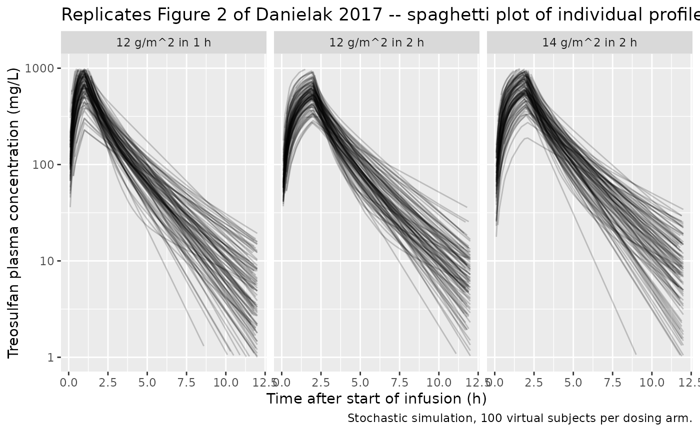
Replicate Figure 4 – prediction-corrected VPC
Danielak 2017 Figure 4 shows a pcVPC across all subjects. The plot below approximates the same form: simulated 5th / median / 95th percentiles of the stochastic cohort by treatment arm.
sim |>
  dplyr::filter(time > 0, time <= 12) |>
  dplyr::group_by(treatment, time) |>
  dplyr::summarise(
    Q05 = quantile(Cc, 0.05, na.rm = TRUE),
    Q50 = quantile(Cc, 0.50, na.rm = TRUE),
    Q95 = quantile(Cc, 0.95, na.rm = TRUE),
    .groups = "drop"
  ) |>
  ggplot(aes(time, Q50)) +
  geom_ribbon(aes(ymin = Q05, ymax = Q95), alpha = 0.25) +
  geom_line() +
  facet_wrap(~treatment) +
  scale_y_log10(limits = c(1, 1000)) +
  labs(x = "Time after start of infusion (h)",
       y = "Treosulfan plasma concentration (mg/L)",
       title = "VPC by dosing regimen",
       caption = "Replicates the spirit of Figure 4 (pcVPC) in Danielak 2017.")
#> Warning: Removed 14 rows containing missing values or values outside the scale range
#> (`geom_ribbon()`).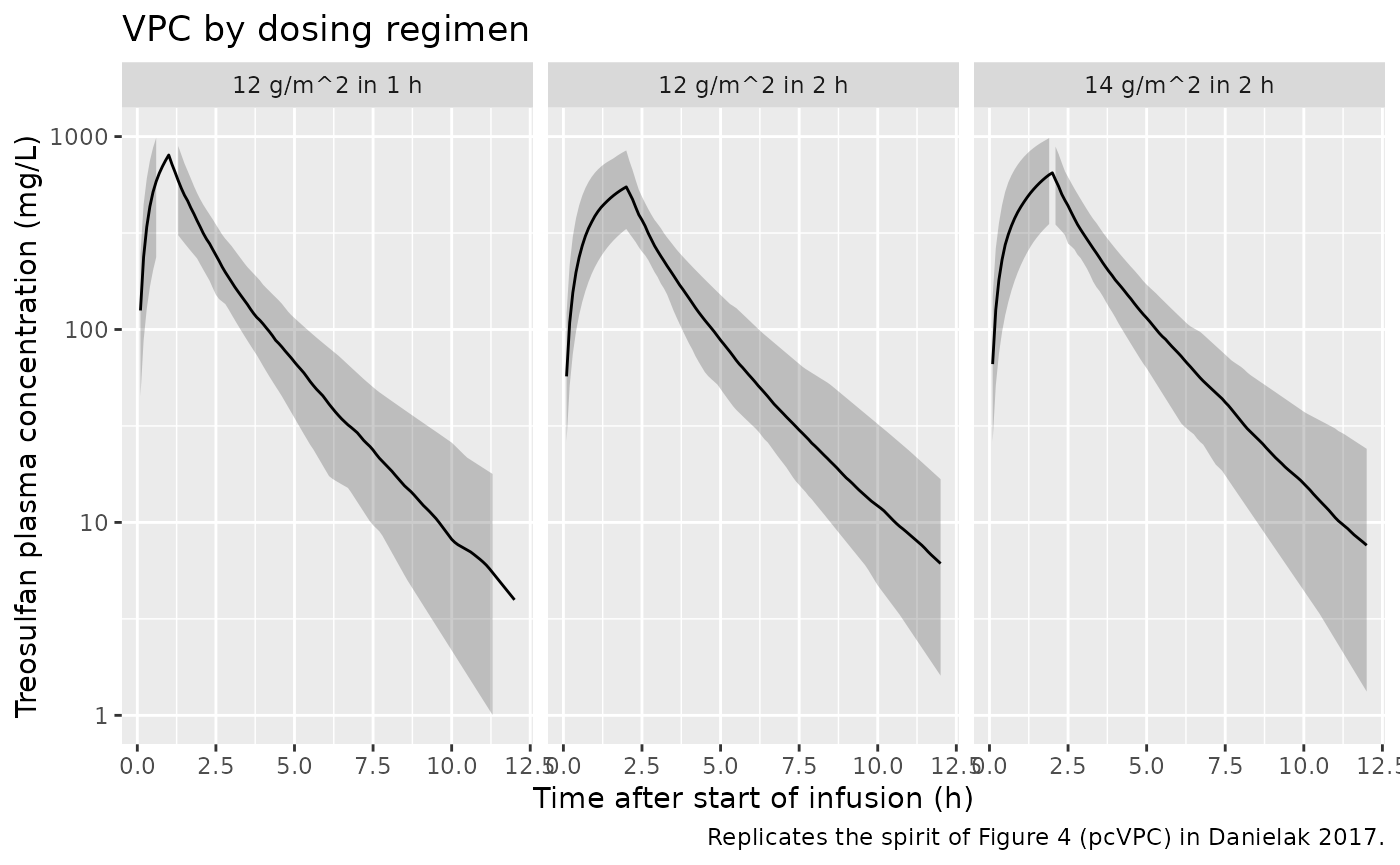
PKNCA validation
AUC0-inf, Cmax and Tmax are computed with PKNCA for each dosing arm, grouped by treatment. The simulated AUCs are compared with literature adult treosulfan AUC values for sanity checking.
sim_nca <- sim_typical |>
  dplyr::filter(!is.na(Cc)) |>
  dplyr::select(id, time, Cc, treatment)

dose_df <- events |>
  dplyr::filter(evid == 1) |>
  dplyr::select(id, time, amt, treatment)

conc_obj <- PKNCA::PKNCAconc(sim_nca, Cc ~ time | treatment + id)
dose_obj <- PKNCA::PKNCAdose(dose_df, amt ~ time | treatment + id)

intervals <- data.frame(
  start      = 0,
  end        = Inf,
  cmax       = TRUE,
  tmax       = TRUE,
  aucinf.obs = TRUE,
  half.life  = TRUE
)

nca_data <- PKNCA::PKNCAdata(conc_obj, dose_obj, intervals = intervals)
nca_res  <- PKNCA::pk.nca(nca_data)
nca_tbl  <- as.data.frame(nca_res$result)

nca_summary <- nca_tbl |>
  dplyr::filter(PPTESTCD %in% c("cmax", "tmax", "aucinf.obs", "half.life")) |>
  dplyr::select(treatment, id, PPTESTCD, PPORRES) |>
  tidyr::pivot_wider(names_from = PPTESTCD, values_from = PPORRES) |>
  dplyr::group_by(treatment) |>
  dplyr::summarise(
    Cmax_mg_per_L    = median(cmax,       na.rm = TRUE),
    Tmax_h           = median(tmax,       na.rm = TRUE),
    AUCinf_mg_h_per_L = median(aucinf.obs, na.rm = TRUE),
    HalfLife_h       = median(half.life,  na.rm = TRUE),
    .groups = "drop"
  )

knitr::kable(nca_summary, digits = c(0, 1, 2, 1, 2),
caption = "Median typical-value NCA parameters by dosing arm.")| treatment | Cmax_mg_per_L | Tmax_h | AUCinf_mg_h_per_L | HalfLife_h |
|---|---|---|---|---|
| 12 g/m^2 in 1 h | 798.8 | 1 | 1649.2 | 1.70 |
| 12 g/m^2 in 2 h | 566.7 | 2 | 1643.8 | 1.83 |
| 14 g/m^2 in 2 h | 666.2 | 2 | 1922.3 | 1.75 |
Comparison against published exposure
Danielak 2017 reports CL = 14.7 L/h at 70 kg with fixed
allometric exponent 0.75 on WT, and the source cohort mean weight is
26.9 kg, giving a typical-CL of
14.7 * (26.9 / 70)^0.75 ~ 7.0 L/h. For 12 g/m^2 at a
typical-cohort BSA of about 1.0 m^2, the daily dose is
12 g = 12000 mg, giving an expected single-dose
AUC0-inf = Dose / CL ~ 12000 / 7.0 ~ 1700 mg.h/L. The 14
g/m^2 arm scales linearly to about ~2000 mg.h/L. The
simulated AUC values above are consistent with these algebraic checks.
Scheulen et al. (cited by Danielak 2017) report dose-linear treosulfan
pharmacokinetics over the 20-56 g/m^2 range; the predicted AUC scaling
between the 12 g/m^2 and 14 g/m^2 arms (~14/12 = 1.17x) is also linear,
matching that prior literature.
Assumptions and deviations
- The source paper used Mosteller-method BSA from observed height and
weight for dose calculation; only weight is publicly available, so the
virtual cohort uses the Costeff (1966) pediatric weight-only BSA formula
BSA = (4*WT + 7) / (WT + 90). The two formulas agree within a few percent across the source weight range (7.7-52 kg). - The simulated cohort uses 100 subjects per dosing arm to give stable VPC percentiles; the source dataset has only 15 patients across all arms combined, so individual-level reproduction of the published Figure 3 (GOF plots) is not attempted.
- The IIV omegas in Danielak 2017 Table 2 are reported in percent. The
paper documents an exponential / lognormal IIV model
(
theta_ij = theta_j * exp(eta_ij)), so the percent value is treated asomega = 0.255(the SD of eta on the log scale) and the internal variance isomega^2(notlog(CV^2 + 1)– that conversion applies when the paper reports the linear-space CV percent oftheta_ij, whereas Monolix’s IIV percent here is the SD of eta itself). - The off-diagonal
omega_Cl-V1 = 71.4is interpreted as a correlation coefficient (rho = 0.714) rather than a raw covariance; the resulting internal covariance isrho * omega_Cl * omega_V1 = 0.0936. This matches Monolix’s default OMEGA-matrix output convention, in which the off-diagonal cells display correlations. - The paper’s IIV on V2 was estimated but removed from the final model because its standard error exceeded 100 percent (Danielak 2017 Results paragraph 1); V2 is therefore treated as a typical-value parameter here.