Isoniazid (Horita 2018)
Source:vignettes/articles/Horita_2018_isoniazid.Rmd
Horita_2018_isoniazid.RmdModel and source
- Citation: Horita Y, Alsultan A, Kwara A, Antwi S, Enimil A, Ortsin A, Dompreh A, Yang H, Wiesner L, Peloquin CA. Evaluation of the Adequacy of WHO Revised Dosages of the First-Line Antituberculosis Drugs in Children with Tuberculosis Using Population Pharmacokinetic Modeling and Simulations. Antimicrob Agents Chemother. 2018;62(9):e00008-18. doi:10.1128/AAC.00008-18
- Description: Two-compartment population pharmacokinetic model with first-order absorption and linear elimination for oral isoniazid in Ghanaian children with active tuberculosis (Horita 2018); NAT2 slow-vs-nonslow acetylator phenotype on apparent oral clearance with separate typical-value clearances and separate IIV omegas; allometric weight scaling on CL/F and Q/F (fixed 0.75) and V1/F and V2/F (fixed 1.0) normalised to the cohort median 14.3 kg.
- Article: https://doi.org/10.1128/AAC.00008-18
Population
The model was developed from 113 Ghanaian children with active tuberculosis enrolled at Komfo Anokye Teaching Hospital, Kumasi, Ghana between October 2012 and August 2015 (ClinicalTrials.gov NCT01687504). The cohort spans 3 months to 14 years of age (median 5.00 years, IQR 2.17 to 8.25) and 5 to 30 kg in body weight (median 14.3 kg). NAT2 genotype distribution in the cohort (Table 1): 51 slow acetylators, 50 intermediate, 12 rapid (45.1% slow). 561 isoniazid concentration-time data points were available; 109 below-LLOQ values were left-censored and analyzed via the SAEM algorithm in MonolixSuite2016R1.
Children received isoniazid 7-15 mg/kg orally daily (median 11.0 mg/kg, IQR 9.06-12.8) as part of the standard four-drug anti-TB regimen. PK sampling was performed at steady state with blood samples at 0, 1, 2, 4, and 8 hours postdose. INH was quantified by LC-MS/MS over the analytical range 0.0977 to 26 ug/mL.
The same information is available programmatically via
readModelDb("Horita_2018_isoniazid")$population.
Source trace
| Equation / parameter | Value | Source location |
|---|---|---|
| Structural model: 2-compartment with first-order absorption | – | Results “INH” paragraph 1; Table 2 |
ka (first-order absorption rate, capped at 6.0) |
4.23 1/h | Table 2 |
CL/F slow acetylators (typical at WT = 14.3 kg) |
4.44 L/h | Table 2 |
CL/F nonslow acetylators (typical at WT = 14.3 kg) |
8.08 L/h | Table 2 |
V1/F (typical at WT = 14.3 kg) |
16.6 L | Table 2 |
Q/F (typical at WT = 14.3 kg) |
8.46 L/h | Table 2 |
V2/F (typical at WT = 14.3 kg) |
1.07 L | Table 2 |
| Allometric exponent on CL/F and Q/F | 0.75 (fixed) | Results “INH” paragraph 1 |
| Allometric exponent on V1/F and V2/F | 1.0 (fixed) | Results “INH” paragraph 1 |
| IIV on ka (omega) | 0.567 (61.6% CV) | Table 2 |
| IIV on CL/F slow (omega) | 0.324 (33.3% CV) | Table 2 |
| IIV on CL/F nonslow (omega) | 0.480 (50.9% CV) | Table 2 |
| IIV on V1/F (omega) | 0.241 (24.5% CV) | Table 2 |
| IIV on Q/F (omega) | 0.637 (70.7% CV) | Table 2 |
| IIV on V2/F (omega) | 1.900 (599.7% CV) | Table 2 |
| Residual error: constant a | 0.0393 ug/mL | Table 2 |
| Residual error: slope b | 0.193 (fraction) | Table 2 |
| NAT2 covariate effect on CL/F: slow vs nonslow phenotype | – | Results “INH” paragraph 1 |
Virtual cohort
The simulated cohort below reflects the Horita 2018 Table 1 weight-band structure with the NAT2 genotype distribution stratified into slow (45.1%) vs nonslow (54.9%) groups.
set.seed(20260526)

weight_bands <- tibble::tibble(
  band = c("5-7 kg", "8-14 kg", "15-20 kg", "21-30 kg"),
  weight_median = c(6.45, 12.5, 17.7, 22.4),
  dose_mg = c(60, 90, 120, 210),  # Horita 2018 Table 3 doses achieving 90% Cmax 3 ug/mL TA
  band_idx = seq_len(4)
)

n_per_band <- 100L  # 50 slow + 50 nonslow per band
make_cohort <- function(band_idx, n, id_offset = 0L) {
  row <- weight_bands[band_idx, ]
  ids <- id_offset + seq_len(n)
  obs_times <- seq(0, 24, by = 0.5)
  # First half (lower IDs) = slow, second half = nonslow
  nat2_assignment <- rep(c(1L, 0L), each = n / 2L)
  ev <- rxode2::et(amt = row$dose_mg, time = 0, cmt = "depot") |>
    rxode2::et(obs_times) |>
    rxode2::et(id = ids) |>
    as.data.frame()
  ev$WT <- row$weight_median
  ev$band <- row$band
  ev$NAT2_SLOW <- nat2_assignment[match(ev$id, ids)]
  ev$nat2_group <- ifelse(ev$NAT2_SLOW == 1L, "slow", "nonslow")
  ev
}

events <- dplyr::bind_rows(
  make_cohort(1L, n_per_band, id_offset =   0L),
  make_cohort(2L, n_per_band, id_offset = 200L),
  make_cohort(3L, n_per_band, id_offset = 400L),
  make_cohort(4L, n_per_band, id_offset = 600L)
)
stopifnot(!anyDuplicated(unique(events[, c("id", "time", "evid")])))
Simulation
mod <- readModelDb("Horita_2018_isoniazid")
sim <- rxode2::rxSolve(mod, events = events, keep = c("band", "WT", "NAT2_SLOW", "nat2_group"))
#> ℹ parameter labels from comments will be replaced by 'label()'
#> Warning: some etas defaulted to non-mu referenced, possible parsing error: etalcl_nonslow
#> as a work-around try putting the mu-referenced expression on a simple line
Replicate published figures
sim_cmax <- sim |>
  dplyr::filter(time <= 24, !is.na(Cc)) |>
  dplyr::group_by(id, band, nat2_group) |>
  dplyr::summarise(cmax = max(Cc), .groups = "drop")

ggplot(sim_cmax, aes(x = band, y = cmax, fill = nat2_group)) +
  geom_boxplot(outlier.size = 0.5) +
  geom_hline(yintercept = 3, linetype = "dashed", colour = "red") +
  labs(x = "Weight band",
       y = "Simulated steady-state Cmax (ug/mL)",
       title = "Isoniazid steady-state Cmax by weight band and NAT2 genotype",
       caption = "Replicates Horita 2018 Figure 5A. Dashed line: paediatric target 3 ug/mL.",
       fill = "NAT2")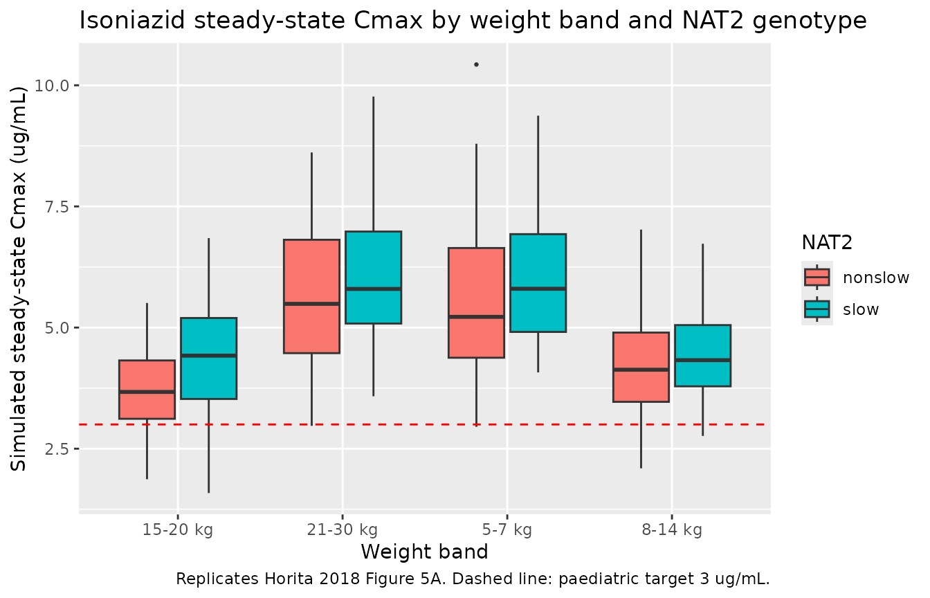
Replicates Figure 5 of Horita 2018 (isoniazid Cmax and AUC by weight band and NAT2 genotype).
PKNCA validation
sim_pk <- sim |>
  dplyr::filter(!is.na(Cc), time <= 24) |>
  dplyr::select(id, time, Cc, band, nat2_group) |>
  dplyr::mutate(group = paste(band, nat2_group, sep = "/"))

conc_obj <- PKNCA::PKNCAconc(sim_pk, Cc ~ time | group + id)
#> Warning in assert_conc(conc, any_missing_conc = any_missing_conc): Negative
#> concentrations found

dose_df <- events |>
  dplyr::filter(evid == 1) |>
  dplyr::mutate(group = paste(band, nat2_group, sep = "/")) |>
  dplyr::select(id, time, amt, group) |>
  dplyr::distinct()

dose_obj <- PKNCA::PKNCAdose(dose_df, amt ~ time | group + id)

intervals <- data.frame(
  start      = 0,
  end        = 24,
  cmax       = TRUE,
  tmax       = TRUE,
  auclast    = TRUE
)

nca_data <- PKNCA::PKNCAdata(conc_obj, dose_obj, intervals = intervals)
nca_res  <- PKNCA::pk.nca(nca_data)
#> Warning in assert_conc(conc, any_missing_conc = any_missing_conc): Negative
#> concentrations found
#> Warning in log(conc.2/conc.1): NaNs produced
#> Warning in assert_conc(conc = conc): Negative concentrations found
#> Warning in assert_conc(conc, any_missing_conc = any_missing_conc): Negative
#> concentrations found
#> Warning in assert_conc(conc, any_missing_conc = any_missing_conc): Negative
#> concentrations found
#> Warning in log(conc.2/conc.1): NaNs produced
#> Warning in assert_conc(conc = conc): Negative concentrations found
#> Warning in assert_conc(conc, any_missing_conc = any_missing_conc): Negative
#> concentrations found

nca_summary <- summary(nca_res)
knitr::kable(nca_summary, caption = "Simulated NCA parameters by weight band and NAT2 genotype (Horita 2018 isoniazid).")| start | end | group | N | auclast | cmax | tmax |
|---|---|---|---|---|---|---|
| 0 | 24 | 15-20 kg/nonslow | 50 | 12.6 [57.2] | 3.63 [24.0] | 0.500 [0.500, 1.50] |
| 0 | 24 | 15-20 kg/slow | 50 | 21.2 [36.2] | 4.20 [32.0] | 1.00 [0.500, 2.00] |
| 0 | 24 | 21-30 kg/nonslow | 50 | 18.0 [42.4], n=49 | 5.44 [28.4] | 0.500 [0.500, 2.00] |
| 0 | 24 | 21-30 kg/slow | 50 | 30.9 [31.2] | 5.96 [24.0] | 0.500 [0.500, 2.00] |
| 0 | 24 | 5-7 kg/nonslow | 50 | 13.1 [47.6], n=49 | 5.24 [31.8] | 0.500 [0.500, 1.00] |
| 0 | 24 | 5-7 kg/slow | 50 | 22.5 [40.7] | 5.90 [21.6] | 0.500 [0.500, 1.50] |
| 0 | 24 | 8-14 kg/nonslow | 50 | 12.3 [52.1], n=48 | 4.12 [25.5] | 0.500 [0.500, 1.50] |
| 0 | 24 | 8-14 kg/slow | 50 | 20.1 [31.4] | 4.30 [22.0] | 0.750 [0.500, 1.50] |
Comparison against published NCA
Horita 2018 (Results “INH” paragraph 1; supplementary Table S1) reports the observed cohort-pooled NCA: median dose 10.99 mg/kg (IQR 9.06-12.80), median Cmax 5.70 ug/mL (IQR 4.27-7.47), median AUC0-8 19.44 mg*h/L (IQR 13.29-24.95). Cmax and AUC0-8 were significantly higher in slow acetylators than in nonslow per the cohort post-hoc analysis (Results “INH” paragraph 2 / Table S1 / Discussion paragraph 2): slow-group simulated median AUC tau is ~1.8 times higher than nonslow per Horita 2018 Discussion.
Assumptions and deviations
- Reference weight 14.3 kg. See the rifampicin vignette for the reference-weight derivation; the same 14.3 kg cohort median applies to all four Horita 2018 drug models.
-
NAT2 encoding. The Horita 2018 source uses a
three-level NAT2 genotype column (slow / intermediate / rapid) and pools
intermediate + rapid as “nonslow” because the NCA post-hoc test showed
no significant differences between intermediate and rapid in CL/F or
AUC0-8 (Results “INH” paragraph 1). The package encodes this binary
phenotype via the general-scope canonical
NAT2_SLOW(1 = slow, 0 = nonslow). The two typical-value clearanceslcl_slow = log(4.44)andlcl_nonslow = log(8.08)and their separate IIV omegas (0.324, 0.480) are selected per-subject insidemodel()viaNAT2_SLOW. -
Per-NAT2-group IIV variances. Horita 2018 Table 2
reports separate omega values for the slow and nonslow acetylator groups
(0.324 vs 0.480), corresponding to Monolix’s “different parameter per
category” option. The model file encodes both omegas; each subject’s
prediction uses exactly one of the two etas based on its
NAT2_SLOWvalue. nlmixr2 generates draws for both etas per subject; only the selected eta enters the prediction. This may generate a “non-mu referenced” parser warning during model load – the warning is benign for simulation use of the model and applies only to mu-referenced fitting workflows. - Combined residual error mapped via the Pythagorean (combined-2) form. See the rifampicin vignette for the rationale.
- Simulated cohort. The per-band doses are taken from Horita 2018 Table 3 (“AUC 0-24 11.95 mg*h/L target attainment dose, Nonslow column”) to reproduce Figure 5 and Table 3.