L-glutamine (Sadaf 2024)
Source:vignettes/articles/Sadaf_2024_glutamine.Rmd
Sadaf_2024_glutamine.RmdModel and source
- Citation: Sadaf A, Dong M, Pfeiffer A, Latham T, Kalfa T, Vinks AA, Ware RE, Quinn CT. A Population Pharmacokinetic Analysis of L-Glutamine Exposure in Patients with Sickle Cell Disease: Evaluation of Dose and Food Effects. Clin Pharmacokinet. 2024;63(3):357-365. doi:10.1007/s40262-024-01349-4.
- Description: One-compartment population PK model with first-order absorption for oral L-glutamine (Endari) in children and adults with sickle cell disease and in healthy adult volunteers (Sadaf 2024). The model is fitted to baseline-subtracted plasma L-glutamine, i.e. the exogenous increment above each participant’s own endogenous pre-dose concentration, so the predicted Cc is zero before the first dose. Apparent oral clearance and apparent central volume are allometrically scaled to body weight with the theoretical exponents 0.75 and 1 (70 kg reference). Apparent clearance falls as the pre-dose endogenous L-glutamine baseline rises (power -0.96, reference 683 umol/L), interpreted as competition between endogenous and exogenous glutamine for elimination. Apparent volume rises with the administered dose per kg (power 0.27, reference 0.1 g/kg), which is how the paper captures the capacity-limited, less-than-dose-proportional rise in exposure seen at 0.3 and 0.6 g/kg after a Michaelis-Menten base model proved unstable. Inter-occasion variability is carried on clearance across the four study visits; inter-individual variability on clearance and on the absorption rate constant, and the additive residual error, were all held at zero in the published final model.
- Article: https://doi.org/10.1007/s40262-024-01349-4
- Trial registration: NCT04684381
L-glutamine (Endari) was approved by the FDA in 2017 to reduce acute complications of sickle cell disease, but the approved 0.3 g/kg twice-daily regimen was chosen empirically. Sadaf 2024 is the first population PK analysis of L-glutamine in sickle cell disease and the first PK study of multiple-dose, long-term oral therapy.
The distinguishing feature of this model is that L-glutamine is
endogenous: it is the most abundant free amino acid in
plasma and every participant already carries several hundred umol/L of
it before the first dose. The authors handled this by subtracting each
participant’s own pre-dose baseline from every measurement and fitting
the increment attributable to the dose. The packaged model
therefore predicts the exogenous increment, and Cc is zero
before the first dose. To recover a measured plasma concentration, add
the subject’s GLN_BL back on.
Population
Twelve participants completed the analysis population of a single-centre, open-label, dose-ascending phase IV trial run at Cincinnati Children’s Hospital Medical Center between January and June 2021, contributing 400 plasma L-glutamine concentrations. They were allocated to three groups of four: paediatric sickle cell disease (age < 18 years), adult sickle cell disease, and healthy adult volunteers. Overall the cohort spanned 6.8-43.8 years and 30.3-119.1 kg, and two thirds were female. Among the eight participants with sickle cell disease, genotypes were evenly split (four homozygous HbSS, four HbSC) as was hydroxyurea use. Healthy volunteers had normal haemoglobin profiles and blood counts. Fifteen participants were enrolled; the three who did not complete at least the third study visit were withdrawn and excluded.
Each participant received three ascending dose levels over three consecutive weeks: 0.1 g/kg twice daily, 0.3 g/kg twice daily, and 0.6 g/kg once daily, dissolved in 120 mL of water. Sampling was pre-dose and at 30, 60, 120, 180, and 240 minutes after the morning dose at each of four study visits. Doses were given either fasting or after a standardised meal so that a food effect could be tested.
Baseline demographics are Sadaf 2024 Table 1, reported per allocation group:
tibble::tribble(
  ~Group,                ~N, ~`Age (years)`,      ~`Weight (kg)`,        ~`Baseline L-glutamine (umol/L)`,
  "Paediatric SCD",      4L, "12.0 (6.8-15.1)",   "64.3 (30.3-101.5)",   "571 (406-720)",
  "Adult SCD",           4L, "23.5 (20.4-29.3)",  "63.45 (49.3-72.8)",   "625 (491-758)",
  "Healthy volunteers",  4L, "37.3 (29.6-43.8)",  "105.1 (67.5-119.1)",  "531 (364-756)"
) |>
knitr::kable(caption = "Sadaf 2024 Table 1: mean (min-max) by allocation group.")| Group | N | Age (years) | Weight (kg) | Baseline L-glutamine (umol/L) |
|---|---|---|---|---|
| Paediatric SCD | 4 | 12.0 (6.8-15.1) | 64.3 (30.3-101.5) | 571 (406-720) |
| Adult SCD | 4 | 23.5 (20.4-29.3) | 63.45 (49.3-72.8) | 625 (491-758) |
| Healthy volunteers | 4 | 37.3 (29.6-43.8) | 105.1 (67.5-119.1) | 531 (364-756) |
The same information is available programmatically via
readModelDb("Sadaf_2024_glutamine")()$population.
Source trace
The per-parameter origin is recorded as an in-file comment next to
each ini() entry in
inst/modeldb/specificDrugs/Sadaf_2024_glutamine.R. The
table below collects them in one place for review. Every value comes
from Sadaf 2024 Table 2 or from the numbered equations in Methods 2.6;
nothing was digitised from a figure, inferred from a related
publication, or supplied by correspondence.
| Equation / parameter | Value | Source location |
|---|---|---|
lka |
log(0.91) 1/h |
Table 2, KA = 0.91 (RSE 6.4%; bootstrap 0.78-0.99) |
lcl |
log(78.5) L/h per 70 kg |
Table 2, theta1 = 78.5 (RSE 7.6%; bootstrap
67.1-91.2) |
lvc |
log(52.3) L per 70 kg |
Table 2, theta3 = 52.3 (RSE 19.5%; bootstrap
30.9-69.9) |
e_wt_cl |
fixed(0.75) |
Eq. 3 (“power is the coefficient set at 0.75 for CL/F”); printed as
a literal exponent in the Table 2 CLi equation |
e_wt_vc |
fixed(1) |
Eq. 3 (“… and 1 for V/F”); printed as a literal exponent in the
Table 2 Vi equation |
e_gln_bl_cl |
-0.96 |
Table 2, theta2 (RSE 19.8%; bootstrap -1.3 to
-0.4) |
e_dose_gln_gkg_vc |
0.27 |
Table 2, theta4 (RSE 45.0%; bootstrap 0.09-0.60) |
etalcl |
fixed(0) |
Table 2, “Inter-patient variability (variance)”, IIV CL = “Fixed to 0” |
etalvc |
0.078 (variance) |
Table 2, IIV V (RSE 19.7%; bootstrap 0.004-0.226) |
etalka |
fixed(0) |
Table 2, IIV Ka = “Fixed to 0” |
etaiov_cl_1..4 |
0.081 (variance) |
Table 2, “Inter-occasion variability (variance)”, IOV CL (RSE 36.4%; bootstrap 0.028-0.144); four occasions per Methods 2.6.1 |
propSd |
0.7 = sqrt(0.49)
|
Table 2, “Residual variability (variance)”, Prop.Err. = 0.49 (RSE 10.9%; bootstrap 0.39-0.59) |
| additive residual | omitted | Table 2, Add.Err. = “Fixed to 0”; Eq. 2 as printed is
Y = Cpred * (1 + eps_prop)
|
GLN_BL reference 683 umol/L |
n/a | Table 2 footnote: “Glu_BSLstardard standard glutamine baseline concentration (683 umol/L)” |
DOSE_GLN_GKG reference 0.1 g/kg |
n/a | Table 2 Vi equation,
(DOSE per kg/0.1)
|
Exponential IIV, Pi = Ppop * exp(eta_i)
|
n/a | Eq. 1 |
Power covariate form,
Pi = Ppop * (COVcon/COVmedian)^theta
|
n/a | Eq. 5 |
| One-compartment, first-order absorption and disposition | n/a | Results 3.3, “a one-compartment model with first-order input and disposition was found to outperform other base models examined” |
| Baseline subtraction of endogenous L-glutamine | n/a | Methods 2.6.1, “the individual baseline l-glutamine concentration was subtracted from each l-glutamine measurement” |
Three of the reported quantities are variances, not
standard deviations or CV%: Table 2 heads the three random-effect blocks
“Inter-patient variability (variance)”, “Inter-occasion variability
(variance)”, and “Residual variability (variance)”. The IIV and IOV
entries are therefore carried into ini() unchanged (rxode2
~ declarations take variances), while propSd
is a standard deviation and is entered as sqrt(0.49) = 0.7.
Reading 0.49 as an SD instead would understate the residual error by
30%, and reading the IIV variances as CV% would overstate them by an
order of magnitude, so this is the single most consequential
transcription decision in the file.
Virtual cohort
Original observed data are not publicly available. The cohort below draws weights and pre-dose L-glutamine baselines from the three allocation groups of Table 1, in the 4:4:4 proportion of the study, using truncated normals whose means match the reported group means and whose spread is set so that the reported min-max spans roughly four standard deviations.
Every virtual participant receives all three dose levels, mirroring
the crossover-like ascending-dose design. Arms are given disjoint ID
ranges because rxSolve treats id as the
subject key.
set.seed(20240224)

n_per_arm <- 100L
mw_gln    <- 146.14  # g/mol, L-glutamine

rtnorm <- function(n, mean, lo, hi) {
  pmin(pmax(stats::rnorm(n, mean, (hi - lo) / 4), lo), hi)
}

# Per-subject covariates, drawn once and reused across the three dose arms so
# the design is paired, as in the trial.
group_levels <- c("Paediatric SCD", "Adult SCD", "Healthy volunteer")
subjects <- tibble::tibble(
  subject = seq_len(n_per_arm),
  group   = sample(group_levels, n_per_arm, replace = TRUE)
) |>
  mutate(
    WT = case_when(
      group == "Paediatric SCD"    ~ rtnorm(n(),  64.30,  30.3, 101.5),
      group == "Adult SCD"         ~ rtnorm(n(),  63.45,  49.3,  72.8),
      group == "Healthy volunteer" ~ rtnorm(n(), 105.10,  67.5, 119.1)
    ),
    GLN_BL = case_when(
      group == "Paediatric SCD"    ~ rtnorm(n(), 571, 406, 720),
      group == "Adult SCD"         ~ rtnorm(n(), 625, 491, 758),
      group == "Healthy volunteer" ~ rtnorm(n(), 531, 364, 756)
    )
  )

# Observation grid: the paper's nominal sampling times (0, 30, 60, 120, 180,
# 240 min) plus a dense grid so the concentration-time figure is smooth.
obs_dense    <- sort(unique(c(seq(0, 6, by = 0.05))))
obs_nominal  <- c(0, 0.5, 1, 2, 3, 4)

make_arm <- function(gkg, occ, id_offset) {
  s <- subjects |>
    mutate(
      id           = id_offset + subject,
      DOSE_GLN_GKG = gkg,
      OCC          = occ,
      treatment    = paste0(format(gkg, nsmall = 1), " g/kg"),
      # Dose amount in umol so that central (umol) / vc (L) is umol/L.
      amt_umol     = gkg * WT / mw_gln * 1e6
    )
  doses <- s |>
    mutate(time = 0, amt = amt_umol, evid = 1L, cmt = "depot")
  obs <- s |>
    tidyr::crossing(time = obs_dense) |>
    mutate(amt = NA_real_, evid = 0L, cmt = "central")
  bind_rows(doses, obs) |>
    select(id, subject, group, time, amt, evid, cmt,
           WT, GLN_BL, DOSE_GLN_GKG, OCC, treatment) |>
    arrange(id, time, desc(evid))
}

events <- bind_rows(
  make_arm(0.1, 1L, id_offset =              0L),
  make_arm(0.3, 2L, id_offset =     n_per_arm),
  make_arm(0.6, 3L, id_offset = 2L * n_per_arm)
)

stopifnot(!anyDuplicated(unique(events[, c("id", "time", "evid")])))
stopifnot(dplyr::n_distinct(events$id) == 3L * n_per_arm)
The OCC column multiplexes the four inter-occasion etas
on log-CL/F. Because Sadaf 2024 reports a single IOV variance shared by
all four occasions, the occasion indices are exchangeable: assigning
arms to occasions 1, 2, 3 rather than to some other permutation changes
nothing about the predicted distribution.
Simulation
mod <- readModelDb("Sadaf_2024_glutamine")

sim <- rxode2::rxSolve(
  mod,
  events = events,
  keep   = c("treatment", "group", "WT", "GLN_BL")
) |>
  as.data.frame()
#> ℹ parameter labels from comments will be replaced by 'label()'
#> Warning: some etas defaulted to non-mu referenced, possible parsing error: etaiov_cl_1, etaiov_cl_2, etaiov_cl_3, etaiov_cl_4
#> as a work-around try putting the mu-referenced expression on a simple line
#> ℹ omega/sigma items treated as zero: 'etalcl', 'etalka'

# rxSolve has been observed to silently drop subjects; assert the count.
stopifnot(dplyr::n_distinct(sim$id) == 3L * n_per_arm)
For the typical-value predictions used to replicate Figure 3, the random effects are zeroed:
mod_typical <- rxode2::zeroRe(mod)
#> ℹ parameter labels from comments will be replaced by 'label()'
#> Warning: some etas defaulted to non-mu referenced, possible parsing error: etaiov_cl_1, etaiov_cl_2, etaiov_cl_3, etaiov_cl_4
#> as a work-around try putting the mu-referenced expression on a simple line
#> Warning: some etas defaulted to non-mu referenced, possible parsing error: etaiov_cl_1, etaiov_cl_2, etaiov_cl_3, etaiov_cl_4
#> as a work-around try putting the mu-referenced expression on a simple line

events_typical <- events |>
  filter(subject == 1L) |>
  mutate(WT = 70, GLN_BL = 683, amt = ifelse(evid == 1L, DOSE_GLN_GKG * 70 / mw_gln * 1e6, amt))

sim_typical <- rxode2::rxSolve(
  mod_typical,
  events = events_typical,
  keep   = c("treatment"),
  omega  = NA
) |>
  as.data.frame()
#> Warning: multi-subject simulation without without 'omega'
Replicate published figures
Figure 2 - concentration-time profiles
Sadaf 2024 Figure 2 plots mean (+/- SD) absolute plasma
L-glutamine against time after dose, with each participant’s visit-1
baseline drawn as a dotted red reference line, to show that
concentrations return to baseline between doses. Because the packaged
model predicts the baseline-subtracted increment, the absolute
concentration is recovered by adding GLN_BL back on.
# Replicates Figure 2 of Sadaf 2024: absolute plasma L-glutamine vs. time.
sim |>
  filter(!is.na(Cc)) |>
  mutate(total = Cc + GLN_BL) |>
  group_by(treatment, time) |>
  summarise(
    mean_total = mean(total),
    lo         = mean(total) - stats::sd(total),
    hi         = mean(total) + stats::sd(total),
    .groups    = "drop"
  ) |>
  ggplot(aes(time, mean_total)) +
  geom_ribbon(aes(ymin = lo, ymax = hi), alpha = 0.2, fill = "grey40") +
  geom_line(linewidth = 0.8) +
  geom_hline(yintercept = mean(subjects$GLN_BL), linetype = "dotted",
             colour = "red", linewidth = 0.6) +
  facet_wrap(~treatment) +
  labs(
    x = "Time after morning dose (h)",
    y = "Plasma L-glutamine (umol/L)",
    title = "Figure 2 - absolute plasma L-glutamine by dose level",
    caption = paste(
      "Replicates Figure 2 of Sadaf 2024. Mean +/- SD of the simulated cohort.",
      "Dotted red line is the cohort mean pre-dose baseline."
    )
  )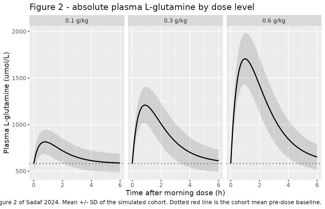
Sadaf 2024 Results 3.2 makes a specific claim about these profiles: “At the lowest dose (0.1 g/kg), l-glutamine concentrations returned to baseline concentrations within 4 hours. However, with 0.3 g/kg or 0.6 g/kg dosing, the plasma l-glutamine concentration remained higher than baseline at 4 h.” That is checkable rather than merely visual, so it is checked:
ret <- sim_typical |>
  filter(!is.na(Cc)) |>
  group_by(treatment) |>
  summarise(
    `Cmax (umol/L)`            = max(Cc),
    `Cc at 4 h (umol/L)`       = Cc[which.min(abs(time - 4))],
    .groups = "drop"
  ) |>
  mutate(`Percent of baseline remaining at 4 h` =
           round(100 * `Cc at 4 h (umol/L)` / 683, 1))

pct <- setNames(ret$`Percent of baseline remaining at 4 h`, ret$treatment)

# Pin the typical-value predictions exactly, so a regression in the model file
# or in rxode2 fails here rather than silently changing the figures.
stopifnot(
  isTRUE(all.equal(unname(pct[c("0.1 g/kg", "0.3 g/kg", "0.6 g/kg")]),
                   c(4.9, 19.5, 46.0), tolerance = 0.01))
)

# The paper's qualitative claim, stated separately from the exact values: at
# 0.1 g/kg the increment at 4 h is a few percent of the endogenous baseline
# (indistinguishable from it on a plot with SD bands), while at 0.3 and
# 0.6 g/kg it is still a substantial and monotonically growing fraction of it.
stopifnot(
  pct[["0.1 g/kg"]] < 10,
  pct[["0.3 g/kg"]] > 15,
  pct[["0.6 g/kg"]] > 40,
  !is.unsorted(pct[c("0.1 g/kg", "0.3 g/kg", "0.6 g/kg")], strictly = TRUE)
)

ret |>
  mutate(across(where(is.numeric), ~ round(.x, 1))) |>
  dplyr::rename("Dose level" = treatment) |>
  knitr::kable(
    caption = paste(
      "Typical-value return to baseline at 4 h. At 0.1 g/kg the remaining",
      "increment is a few percent of the 683 umol/L endogenous baseline;",
      "at 0.3 and 0.6 g/kg it is still a large fraction of it, as",
      "Sadaf 2024 Results 3.2 describes."
    )
)| Dose level | Cmax (umol/L) | Cc at 4 h (umol/L) | Percent of baseline remaining at 4 h |
|---|---|---|---|
| 0.1 g/kg | 256.9 | 33.5 | 4.9 |
| 0.3 g/kg | 676.2 | 133.0 | 19.5 |
| 0.6 g/kg | 1235.8 | 314.0 | 46.0 |
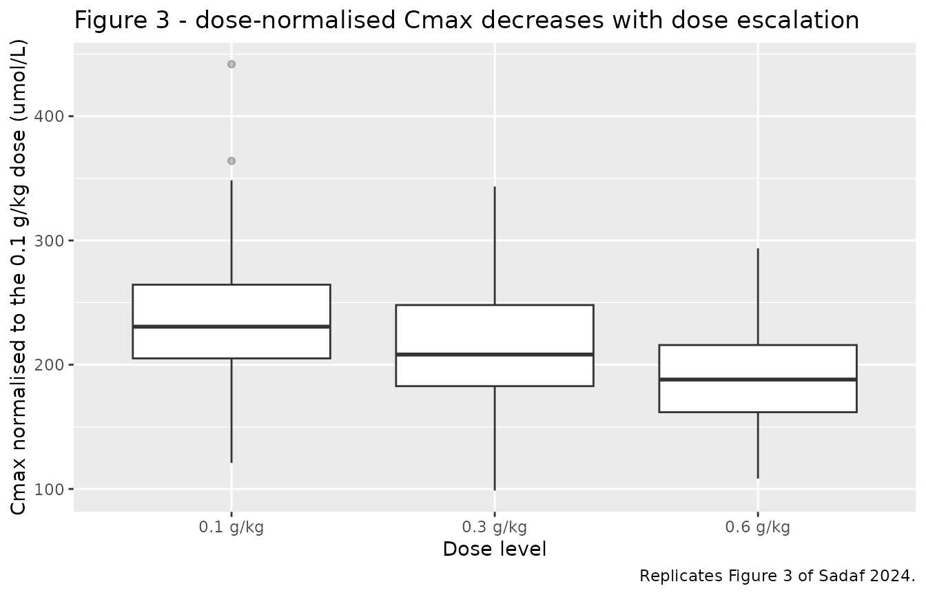
Figure 3 - dose-normalised Cmax falls with dose escalation
This is the paper’s central non-linearity finding, and the reason the model carries dose as a covariate on apparent volume at all.
# Replicates Figure 3 of Sadaf 2024: dose-normalised Cmax vs. dose level.
cmax_norm <- sim |>
  filter(!is.na(Cc)) |>
  group_by(id, treatment, DOSE_GLN_GKG) |>
  summarise(cmax = max(Cc), .groups = "drop") |>
  mutate(cmax_norm = cmax / (DOSE_GLN_GKG / 0.1))

cmax_norm |>
  ggplot(aes(treatment, cmax_norm)) +
  geom_boxplot(outlier.alpha = 0.3) +
  labs(
    x = "Dose level",
    y = "Cmax normalised to the 0.1 g/kg dose (umol/L)",
    title = "Figure 3 - dose-normalised Cmax decreases with dose escalation",
    caption = "Replicates Figure 3 of Sadaf 2024."
  )
sim_typical |>
  filter(!is.na(Cc)) |>
  group_by(treatment) |>
  summarise(
    `Tmax (h)`                 = time[which.max(Cc)],
    `Cmax (umol/L)`            = max(Cc),
    .groups = "drop"
  ) |>
  mutate(
    `Dose multiple of 0.1 g/kg`   = c(1, 3, 6),
    `Dose-normalised Cmax`        = round(`Cmax (umol/L)` / `Dose multiple of 0.1 g/kg`, 1),
    `Cmax (umol/L)`               = round(`Cmax (umol/L)`, 1)
  ) |>
  dplyr::rename("Dose level" = treatment) |>
  knitr::kable(
    caption = paste(
      "Typical-value (70 kg, baseline 683 umol/L) predictions.",
      "Dose-normalised Cmax falls and Tmax rises across the dose range,",
      "reproducing both non-linearity findings of Sadaf 2024."
    )
)| Dose level | Tmax (h) | Cmax (umol/L) | Dose multiple of 0.1 g/kg | Dose-normalised Cmax |
|---|---|---|---|---|
| 0.1 g/kg | 0.85 | 256.9 | 1 | 256.9 |
| 0.3 g/kg | 1.00 | 676.2 | 3 | 225.4 |
| 0.6 g/kg | 1.10 | 1235.8 | 6 | 206.0 |
Two published findings are reproduced here at once. Dose-normalised
Cmax falls monotonically across the three dose levels (Figure 3 and
Results 3.2), and Tmax rises with dose - Sadaf 2024 reports “the Tmax
was higher at the dose of 0.6 g/kg (p < 0.05), indicating slower
absorption at higher doses”. Both fall out of the single
(DOSE per kg / 0.1)^0.27 term on apparent volume: inflating
V/F lowers kel = CL/V, which pushes the model further into flip-flop
kinetics (ka = 0.91 1/h against kel = 1.50, 1.12, and 0.93 1/h at the
three dose levels) and so both depresses and delays the peak. No
separate absorption-rate covariate is needed.
PKNCA validation
The NCA below uses the paper’s own nominal sampling schedule (pre-dose and 30, 60, 120, 180, 240 minutes) rather than the dense grid, so that the comparison against the published NCA is made on comparable data. Like the paper, the NCA is run on the baseline-subtracted concentrations: Sadaf 2024 Methods 2.5 states that “Cmax values were obtained by subtracting baseline concentrations from peak values”.
sim_nca <- sim |>
  filter(!is.na(Cc), time %in% obs_nominal) |>
  select(id, time, Cc, treatment)

# Guarantee a time = 0 row per (id, treatment); pre-dose Cc = 0 is correct for
# this baseline-subtracted, extravascular model.
sim_nca <- bind_rows(
  sim_nca,
  sim_nca |> distinct(id, treatment) |> mutate(time = 0, Cc = 0)
) |>
  distinct(id, treatment, time, .keep_all = TRUE) |>
  arrange(id, treatment, time)

dose_df <- events |>
  filter(evid == 1L) |>
  select(id, time, amt, treatment)

conc_obj <- PKNCA::PKNCAconc(sim_nca, Cc ~ time | treatment + id,
                             concu = "umol/L", timeu = "hr")
dose_obj <- PKNCA::PKNCAdose(dose_df, amt ~ time | treatment + id,
                             doseu = "umol")

intervals <- data.frame(
  start      = 0,
  end        = 4,
  cmax       = TRUE,
  tmax       = TRUE,
  auclast    = TRUE,
  half.life  = TRUE
)

nca_res <- PKNCA::pk.nca(PKNCA::PKNCAdata(conc_obj, dose_obj, intervals = intervals))
#> Warning: Too few points for half-life calculation (min.hl.points=3 with only 2 points)
#> Too few points for half-life calculation (min.hl.points=3 with only 2 points)
#> Too few points for half-life calculation (min.hl.points=3 with only 2 points)
#> Too few points for half-life calculation (min.hl.points=3 with only 2 points)
#> Too few points for half-life calculation (min.hl.points=3 with only 2 points)
summary(nca_res)
#>  Interval Start Interval End treatment   N AUClast (hr*umol/L) Cmax (umol/L)
#>               0            4  0.1 g/kg 100          467 [30.0]    228 [22.1]
#>               0            4  0.3 g/kg 100         1370 [31.5]    616 [22.3]
#>               0            4  0.6 g/kg 100         2640 [26.9]   1110 [20.6]
#>           Tmax (hr)     Half-life (hr)
#>  1.00 [0.500, 1.00]      0.903 [0.162]
#>  1.00 [0.500, 2.00] 1.04 [0.310], n=99
#>  1.00 [0.500, 2.00] 1.11 [0.247], n=96
#>
#> Caption: AUClast, Cmax: geometric mean and geometric coefficient of variation; Tmax: median and range; Half-life: arithmetic mean and standard deviation; N: number of subjects; n: number of measurements included in summary
Comparison against published NCA
Sadaf 2024 reports only two NCA parameters numerically, and reports both pooled across dose levels and visits rather than per dose group: Tmax averaged 1.2 +/- 0.9 h (Results 3.2) and the apparent terminal half-life averaged 1.0 +/- 0.7 h, computed only “from visits when samples were rich enough”. Cmax appears in Figure 3 in dose-normalised form only, with no axis values transcribable as a point estimate, so it cannot enter a numeric comparison. The published values are therefore repeated across the three simulated arms below; the per-arm spread of the simulated values is the informative part.
published <- tibble::tribble(
  ~treatment,  ~tmax, ~half.life,
  "0.1 g/kg",  1.2,   1.0,
  "0.3 g/kg",  1.2,   1.0,
  "0.6 g/kg",  1.2,   1.0
)

cmp <- nlmixr2lib::ncaComparisonTable(
  simulated     = nca_res,
  reference     = published,
  by            = "treatment",
  units         = c(tmax = "h", half.life = "h"),
  tolerance_pct = 20
)

knitr::kable(
  cmp,
  caption = paste(
    "Simulated vs. published NCA. Published values are the pooled",
    "cohort means of Sadaf 2024 Results 3.2, repeated for each arm.",
    "* differs from reference by >20%."
  ),
  align = c("l", "l", "r", "r", "r")
)| NCA parameter | treatment | Reference | Simulated | % diff |
|---|---|---|---|---|
| Tmax (h) | 0.1 g/kg | 1.2 | 1 | -16.7% |
| Tmax (h) | 0.3 g/kg | 1.2 | 1 | -16.7% |
| Tmax (h) | 0.6 g/kg | 1.2 | 1 | -16.7% |
| t½ (h) | 0.1 g/kg | 1 | 0.842 | -15.8% |
| t½ (h) | 0.3 g/kg | 1 | 0.925 | -7.5% |
| t½ (h) | 0.6 g/kg | 1 | 1.07 | +7.3% |
The simulated half-lives (0.84, 0.93, and 1.07 h) bracket the published pooled mean of 1.0 h, and none of the three differs from it by more than 20%. This is worth a note, because a naive reading of the model would not predict it: with CL/F = 78.5 L/h and V/F = 52.3 L the elimination rate constant at the reference dose is 1.50 1/h, implying a disposition half-life of only 0.46 h. But ka = 0.91 1/h is smaller than kel, so the model sits in flip-flop kinetics and the observable terminal slope is governed by absorption rather than elimination, with an asymptotic value of log(2)/0.91 = 0.76 h. The values above run a little longer than that because the paper’s 0-4 h window ends before the profile is purely terminal, and they lengthen with dose because inflating V/F lowers kel toward ka, which flattens the observed decline. That a 1-hour-half-life observation falls out of a model whose disposition half-life is 28 minutes is a meaningful check that absorption and disposition were transcribed into the right roles, and not swapped.
Simulated Tmax runs slightly below the published pooled mean of 1.2 h. Two reasons, both structural rather than a transcription problem. First, the published mean pools all four visits including the 0.6 g/kg visit, whose Tmax the paper explicitly reports as higher; the simulated per-arm values bracket the pooled mean in the same direction. Second, Tmax on the paper’s sparse nominal grid can only take the values 0.5, 1, 2, 3, or 4 h, so a published mean of 1.2 h with an SD of 0.9 h reflects a handful of subjects whose observed peak landed at 2 h or later. No parameter was adjusted to close the gap.
Assumptions and deviations
-
The model predicts the baseline-subtracted increment, not
the measured concentration. Sadaf 2024 Methods 2.6.1 subtracted
each participant’s pre-dose L-glutamine from every measurement before
fitting, assuming the endogenous level is constant.
Ccis therefore zero before the first dose, and a measured plasma concentration isCc + GLN_BL. Users simulating this model to predict laboratory values must add the baseline back on, as the Figure 2 chunk above does. -
GLN_BLdoes double duty. The same per-subject baseline both defines the zero of the concentration scale and enters the CL/F covariate equation. When simulating, one value per subject must be supplied and used consistently for both purposes. - Virtual cohort distributions are assumed. Sadaf 2024 Table 1 reports group means and min-max but no distributional form or correlation structure. Weight and baseline L-glutamine are drawn here as independent truncated normals per allocation group with the spread set so the reported range spans about four SD. In the real cohort the two are almost certainly correlated with age and group, and n = 4 per group makes the reported ranges unstable.
- Occasion-to-dose-level mapping is a presentation choice. The paper defines four occasions (Methods 2.6.1) corresponding to study visits, and Figure 1 carries the visit-by-visit dose and meal schema, but the running text does not state which visit carried which dose level unambiguously (“the dose was increased (visit 2) or continued unchanged (visit 3)”). This vignette assigns the three simulated arms to occasions 1, 2, and 3. Because Table 2 reports a single IOV variance shared across all four occasions, the assignment is exchangeable and does not affect the predicted distribution.
- Cmax could not be compared numerically. Sadaf 2024 presents Cmax only in Figure 3, dose-normalised, with no transcribable axis values, and reports no Cmax table. Only Tmax and half-life entered the comparison table. Consistent with the standing policy, no value was digitised off the figure.
- The published Tmax and half-life are pooled, not per dose level. They are repeated across the three arms in the comparison table above. The paper’s per-dose statement about Tmax (higher at 0.6 g/kg, p < 0.05) is checked separately in the typical-value table under Figure 3.
-
Screened but unretained covariates are documented, not
encoded. Age, height, body surface area, sex, serum creatinine,
haemoglobin genotype, baseline L-glutamate, and meal intake were all
tested by stepwise selection and none was retained (Results 3.3). No
point estimates are published for any of them, so they appear in the
model file’s
covariatesDataExcludedmetadata rather than incovariateData. Note in particular that the meal covariate was not coded as a plain binary: Methods 2.6.2 used 0 for fasting, 0.5 for a snack, 1 for a full meal, and 1.5 for a snack plus a full meal between consecutive measurements. - Allometric exponents are treated as fixed. Eq. 3 states the exponents were “set at” 0.75 and 1, and Table 2 prints them as literal exponents with no estimate, RSE, or bootstrap interval, unlike every estimated theta in the same table. Results 3.3 separately reports that free estimation gave 0.73 and 0.78; those exploratory values are not the final model and are not used here.
- A Michaelis-Menten alternative was tested and rejected by the authors. Results 3.3 reports that a Michaelis-Menten base model was unstable, which is why the observed capacity-limited behaviour is carried by a dose effect on apparent volume instead. The packaged model replicates the authors’ final structure, not the rejected one.
- The parent-metabolite extension was abandoned by the authors. Methods 2.6.1 reports that a simultaneous L-glutamine / L-glutamate model was attempted but the conversion parameter sat near the zero boundary, so L-glutamate is not part of the final model and is not extracted.
Errata and source-quality notes
- Sadaf 2024 Table 1 prints the paediatric age range as “6.8-5.1”, which is not a range. The correct upper bound is 15.1 years: the paediatric group is defined as age < 18 years with a mean of 12.0, and the Abstract and Results give the overall cohort range as 6.8-43.8 years with the healthy-volunteer group topping out at 43.8. The vignette population table above uses 15.1.
- The paper contradicts itself on hydroxyurea use. Table 1 reports
“Yes (1) / No (3)” for the paediatric group and “Yes (2) / No (2)” for
the adult group, i.e. 3 of 8 participants with sickle cell disease on
hydroxyurea, whereas Results 3.1 states that the group had an equal
distribution of “hydroxyurea use (four yes, four no)”. The genotype
counts in the same sentence do agree with Table 1, so the discrepancy is
confined to hydroxyurea. It has no effect on the extraction: hydroxyurea
was not among the covariates screened in Methods 2.6.2, and the model
file’s
populationmetadata records both counts rather than choosing one. - The Table 2 footnote spells the standard-baseline symbol “Glu_BSLstardard”, a typographical variant of “standard”. The value it defines, 683 umol/L, is unambiguous and is the normalisation constant used in the model.
- Table 2’s footnote also glosses “BIO relative bioavailability”, but no BIO parameter appears anywhere in the table or in the model equations. It appears to be a leftover abbreviation; no bioavailability term is extracted.
- Methods 2.6.1 describes the residual error as “a proportional and
additive error model”, but Eq. 2 as typeset is purely proportional,
Y = Cpred * (1 + eps_prop), and Table 2 reports the additive component as “Fixed to 0”. The equation and the table agree with each other, so the model carries a proportional error only; the prose is describing the error model that was tested rather than the one that was retained. - No erratum or corrigendum for this article was found. The article is open access under CC BY-NC 4.0.
- The Electronic Supplementary Material (participant flow diagram, adverse-event table, and goodness-of-fit plots) contains no parameter values needed for the model, so the extraction does not depend on it.