Preclinical rFVIIa + rFVIII animal popPK (Larsen 2018)
Source:vignettes/articles/Larsen_2018_haemophilia_animal_popPK.Rmd
Larsen_2018_haemophilia_animal_popPK.RmdPaper
Larsen MS, Juul RV, Groth AV, Simonsson USH, Kristensen AT, Knudsen T, Agerso H, Kreilgaard M. (2018). Prediction of human pharmacokinetics of activated recombinant factor VII and B-domain truncated factor VIII from animal population pharmacokinetic models of haemophilia. European Journal of Pharmaceutical Sciences 119, 265-273. doi:10.1016/j.ejps.2018.01.035 (PMID: 29369801)
The paper develops eight species-specific population PK models – one for each of the two coagulation factors (activated recombinant factor VII, rFVIIa; and B-domain truncated recombinant factor VIII, rFVIII) times each of four preclinical species (mouse, rat, cynomolgus monkey, beagle / haemophilia A dog). Human plasma concentration-time data from Bysted et al. 2007 (rFVIIa) and Jimenez-Yuste et al. 2015 (rFVIII) were used only for external validation of the animal-scaled predictions; no new human popPK model is developed in Larsen 2018 and none is packaged here.
Each of the eight models is packaged separately (following the “replicate the author’s structure” default – the models were genuinely independent fits), and this vignette walks the paper as a whole.
Models
larsen_stems <- c(
  "Larsen_2018_factorviia_mouse",  "Larsen_2018_factorviia_rat",
  "Larsen_2018_factorviia_monkey", "Larsen_2018_factorviia_dog",
  "Larsen_2018_factorviii_mouse",  "Larsen_2018_factorviii_rat",
  "Larsen_2018_factorviii_monkey", "Larsen_2018_factorviii_dog"
)

meta <- lapply(larsen_stems, function(stem) {
  fn <- readModelDb(stem)
  m  <- fn()
  data.frame(
    model         = stem,
    species       = m$population$species,
    n_subjects    = m$population$n_subjects %||% NA_integer_,
    weight_median = m$population$weight_median %||% NA_character_,
    stringsAsFactors = FALSE
  )
})
meta <- do.call(rbind, meta)
knitr::kable(meta, caption = "The eight species-specific popPK models packaged from Larsen 2018.")| model | species | n_subjects | weight_median |
|---|---|---|---|
| Larsen_2018_factorviia_mouse | mouse (C57BI/6 and NMRI, pooled) | 51 | 0.026 kg |
| Larsen_2018_factorviia_rat | rat (Sprague-Dawley) | 37 | 0.24 kg |
| Larsen_2018_factorviia_monkey | monkey (cynomolgus) | 27 | 2.78 kg |
| Larsen_2018_factorviia_dog | beagle dog | 10 | 12.8 kg |
| Larsen_2018_factorviii_mouse | mouse (FVIII knockout) | 132 | 0.021 kg |
| Larsen_2018_factorviii_rat | rat (Sprague-Dawley) | 60 | 0.32 kg |
| Larsen_2018_factorviii_monkey | monkey (cynomolgus) | 35 | 2.96 kg |
| Larsen_2018_factorviii_dog | dog (haemophilia A) | 3 | 19.55 kg |
Population
The Larsen 2018 preclinical cohort spans 51 mice + 37 rats + 27 monkeys + 10 beagle dogs (rFVIIa arm; Table 1) and 132 mice + 60 rats + 35 monkeys + 3 haemophilia A dogs (rFVIII arm; Table 1). Data originate from 33 studies – historical unpublished in-house Novo Nordisk experiments plus the published studies by Karpf et al. 2011 (glycopegylated rFVIIa variants), Agerso et al. 2011b (rFVIIa in dogs), Elm et al. 2012 (rFVIII in mice), Stennicke et al. 2013 (N8-GP rFVIII in haemophilic mice), and Agerso et al. 2012 (rFVIII in dogs).
All animal experiments used single IV bolus administration. Doses are reported in mass units (ug/kg for rFVIIa; IU/kg for rFVIII); the packaged models take input in activity units (IU for both), so a user simulating rFVIIa must convert dose-mass to activity using the product-specific specific activity.
Human validation cohorts (Bysted 2007 rFVIIa, Jimenez-Yuste 2015 rFVIII) are outside the scope of the packaged animal models.
Source trace
source_trace <- tibble::tribble(
  ~equation_or_parameter,                      ~value,                        ~source_location,
  # rFVIIa mouse ---------------------------------------------------------------
  "rFVIIa mouse V",                            "2.72 mL",                     "Larsen 2018 Table 2, Mouse column",
  "rFVIIa mouse CL",                           "3.2 mL/h",                    "Larsen 2018 Table 2, Mouse column",
  "rFVIIa mouse V2",                           "0.384 mL",                    "Larsen 2018 Table 2, Mouse column",
  "rFVIIa mouse Q",                            "0.244 mL/h",                  "Larsen 2018 Table 2, Mouse column",
  "rFVIIa mouse Cov V,C57BI/6",                "0.588",                       "Larsen 2018 Table 2, Mouse column footnote",
  "rFVIIa mouse Cov CL,C57BI/6",               "0.87",                        "Larsen 2018 Table 2, Mouse column footnote",
  "rFVIIa mouse IIV on CL",                    "7.4% CV",                     "Larsen 2018 Table 2, Mouse column",
  "rFVIIa mouse residual",                     "0.131",                       "Larsen 2018 Table 2, Mouse column",
  # rFVIIa rat ----------------------------------------------------------------
  "rFVIIa rat V",                              "18.6 mL",                     "Larsen 2018 Table 2, Rat column",
  "rFVIIa rat CL",                             "16.5 mL/h",                   "Larsen 2018 Table 2, Rat column",
  "rFVIIa rat V2",                             "2.68 mL",                     "Larsen 2018 Table 2, Rat column",
  "rFVIIa rat Q",                              "1.63 mL/h",                   "Larsen 2018 Table 2, Rat column",
  "rFVIIa rat IIV on V",                       "16.3% CV",                    "Larsen 2018 Table 2, Rat column",
  "rFVIIa rat IIV on CL",                      "14.6% CV",                    "Larsen 2018 Table 2, Rat column",
  "rFVIIa rat residual",                       "0.161",                       "Larsen 2018 Table 2, Rat column",
  # rFVIIa monkey ------------------------------------------------------------
  "rFVIIa monkey V",                           "229 mL",                      "Larsen 2018 Table 2, Monkey column",
  "rFVIIa monkey CL",                          "148 mL/h",                    "Larsen 2018 Table 2, Monkey column",
  "rFVIIa monkey V2",                          "62.1 mL",                     "Larsen 2018 Table 2, Monkey column",
  "rFVIIa monkey Q",                           "42.3 mL/h",                   "Larsen 2018 Table 2, Monkey column",
  "rFVIIa monkey Base FVIIa",                  "0.287 IU/mL",                 "Larsen 2018 Table 2, Monkey column",
  "rFVIIa monkey IIV on V",                    "54.7% CV",                    "Larsen 2018 Table 2, Monkey column",
  "rFVIIa monkey IIV on CL",                   "35.1% CV",                    "Larsen 2018 Table 2, Monkey column",
  "rFVIIa monkey IIV on Base FVIIa",           "42.8% CV",                    "Larsen 2018 Table 2, Monkey column",
  "rFVIIa monkey residual",                    "0.0343",                      "Larsen 2018 Table 2, Monkey column",
  # rFVIIa dog ---------------------------------------------------------------
  "rFVIIa dog V",                              "1300 mL",                     "Larsen 2018 Table 2, Dog column",
  "rFVIIa dog CL",                             "761 mL/h",                    "Larsen 2018 Table 2, Dog column",
  "rFVIIa dog V2",                             "200 mL",                      "Larsen 2018 Table 2, Dog column",
  "rFVIIa dog Q",                              "55.6 mL/h",                   "Larsen 2018 Table 2, Dog column",
  "rFVIIa dog IIV on V",                       "25.8% CV",                    "Larsen 2018 Table 2, Dog column",
  "rFVIIa dog IIV on CL",                      "34.7% CV",                    "Larsen 2018 Table 2, Dog column",
  "rFVIIa dog residual",                       "0.0236",                      "Larsen 2018 Table 2, Dog column",
  # rFVIII mouse -------------------------------------------------------------
  "rFVIII mouse V",                            "0.716 mL",                    "Larsen 2018 Table 3, Mouse column",
  "rFVIII mouse CL",                           "0.0639 mL/h",                 "Larsen 2018 Table 3, Mouse column",
  "rFVIII mouse Cov CL,Female",                "1.24",                        "Larsen 2018 Table 3, Mouse column footnote",
  "rFVIII mouse IIV on CL",                    "19% CV",                      "Larsen 2018 Table 3, Mouse column",
  "rFVIII mouse residual",                     "0.231",                       "Larsen 2018 Table 3, Mouse column",
  # rFVIII rat --------------------------------------------------------------
  "rFVIII rat V",                              "9.52 mL",                     "Larsen 2018 Table 3, Rat column",
  "rFVIII rat CL0",                            "1.89 mL/h",                   "Larsen 2018 Table 3, Rat column",
  "rFVIII rat Base FVIII",                     "1.12 IU/mL",                  "Larsen 2018 Table 3, Rat column",
  "rFVIII rat beta (nonlinear CL slope)",      "0.162 mL/IU",                 "Larsen 2018 Table 3, Rat column (Eq. 1)",
  "rFVIII rat Cov CL,Female",                  "1.39",                        "Larsen 2018 Table 3, Rat column footnote",
  "rFVIII rat IIV on Base FVIII",              "24.2% CV",                    "Larsen 2018 Table 3, Rat column",
  "rFVIII rat residual",                       "0.305",                       "Larsen 2018 Table 3, Rat column",
  # rFVIII monkey ----------------------------------------------------------
  "rFVIII monkey V",                           "145 mL",                      "Larsen 2018 Table 3, Monkey column",
  "rFVIII monkey CL0",                         "13.1 mL/h",                   "Larsen 2018 Table 3, Monkey column",
  "rFVIII monkey Base FVIII",                  "1.75 IU/mL",                  "Larsen 2018 Table 3, Monkey column",
  "rFVIII monkey beta (nonlinear CL slope)",   "0.0355 mL/IU",                "Larsen 2018 Table 3, Monkey column (Eq. 1)",
  "rFVIII monkey IIV on CL",                   "55% CV",                      "Larsen 2018 Table 3, Monkey column",
  "rFVIII monkey IIV on Base FVIII",           "39.5% CV",                    "Larsen 2018 Table 3, Monkey column",
  "rFVIII monkey residual",                    "0.229",                       "Larsen 2018 Table 3, Monkey column",
  # rFVIII dog -------------------------------------------------------------
  "rFVIII dog V",                              "765 mL",                      "Larsen 2018 Table 3, Dog column",
  "rFVIII dog CL",                             "67.7 mL/h",                   "Larsen 2018 Table 3, Dog column",
  "rFVIII dog V2",                             "92.4 mL",                     "Larsen 2018 Table 3, Dog column",
  "rFVIII dog Q",                              "4.92 mL/h",                   "Larsen 2018 Table 3, Dog column",
  "rFVIII dog residual",                       "0.209",                       "Larsen 2018 Table 3, Dog column",
  # Structural equations --------------------------------------------------
  "Allometric scaling (V, V2)",                "exponent 1",                  "Larsen 2018 Eq. 2 (scaling principle I)",
  "Allometric scaling (CL, Q)",                "exponent 0.75",               "Larsen 2018 Eq. 2 (scaling principle I)",
  "Nonlinear CL",                              "CL = CL0 * exp(beta * C)",    "Larsen 2018 Eq. 1 (rat + monkey rFVIII)",
  "Two-compartment ODE (rFVIIa)",              "central + peripheral1",        "Larsen 2018 Sec 2.4",
  "One-compartment ODE (rFVIII mouse/rat/monkey)", "central only",            "Larsen 2018 Sec 3.1",
  "Two-compartment ODE (rFVIII dog)",          "central + peripheral1",        "Larsen 2018 Sec 3.1"
)
knitr::kable(source_trace, caption = "Source-trace: every parameter and structural equation, with its location in Larsen 2018.")| equation_or_parameter | value | source_location |
|---|---|---|
| rFVIIa mouse V | 2.72 mL | Larsen 2018 Table 2, Mouse column |
| rFVIIa mouse CL | 3.2 mL/h | Larsen 2018 Table 2, Mouse column |
| rFVIIa mouse V2 | 0.384 mL | Larsen 2018 Table 2, Mouse column |
| rFVIIa mouse Q | 0.244 mL/h | Larsen 2018 Table 2, Mouse column |
| rFVIIa mouse Cov V,C57BI/6 | 0.588 | Larsen 2018 Table 2, Mouse column footnote |
| rFVIIa mouse Cov CL,C57BI/6 | 0.87 | Larsen 2018 Table 2, Mouse column footnote |
| rFVIIa mouse IIV on CL | 7.4% CV | Larsen 2018 Table 2, Mouse column |
| rFVIIa mouse residual | 0.131 | Larsen 2018 Table 2, Mouse column |
| rFVIIa rat V | 18.6 mL | Larsen 2018 Table 2, Rat column |
| rFVIIa rat CL | 16.5 mL/h | Larsen 2018 Table 2, Rat column |
| rFVIIa rat V2 | 2.68 mL | Larsen 2018 Table 2, Rat column |
| rFVIIa rat Q | 1.63 mL/h | Larsen 2018 Table 2, Rat column |
| rFVIIa rat IIV on V | 16.3% CV | Larsen 2018 Table 2, Rat column |
| rFVIIa rat IIV on CL | 14.6% CV | Larsen 2018 Table 2, Rat column |
| rFVIIa rat residual | 0.161 | Larsen 2018 Table 2, Rat column |
| rFVIIa monkey V | 229 mL | Larsen 2018 Table 2, Monkey column |
| rFVIIa monkey CL | 148 mL/h | Larsen 2018 Table 2, Monkey column |
| rFVIIa monkey V2 | 62.1 mL | Larsen 2018 Table 2, Monkey column |
| rFVIIa monkey Q | 42.3 mL/h | Larsen 2018 Table 2, Monkey column |
| rFVIIa monkey Base FVIIa | 0.287 IU/mL | Larsen 2018 Table 2, Monkey column |
| rFVIIa monkey IIV on V | 54.7% CV | Larsen 2018 Table 2, Monkey column |
| rFVIIa monkey IIV on CL | 35.1% CV | Larsen 2018 Table 2, Monkey column |
| rFVIIa monkey IIV on Base FVIIa | 42.8% CV | Larsen 2018 Table 2, Monkey column |
| rFVIIa monkey residual | 0.0343 | Larsen 2018 Table 2, Monkey column |
| rFVIIa dog V | 1300 mL | Larsen 2018 Table 2, Dog column |
| rFVIIa dog CL | 761 mL/h | Larsen 2018 Table 2, Dog column |
| rFVIIa dog V2 | 200 mL | Larsen 2018 Table 2, Dog column |
| rFVIIa dog Q | 55.6 mL/h | Larsen 2018 Table 2, Dog column |
| rFVIIa dog IIV on V | 25.8% CV | Larsen 2018 Table 2, Dog column |
| rFVIIa dog IIV on CL | 34.7% CV | Larsen 2018 Table 2, Dog column |
| rFVIIa dog residual | 0.0236 | Larsen 2018 Table 2, Dog column |
| rFVIII mouse V | 0.716 mL | Larsen 2018 Table 3, Mouse column |
| rFVIII mouse CL | 0.0639 mL/h | Larsen 2018 Table 3, Mouse column |
| rFVIII mouse Cov CL,Female | 1.24 | Larsen 2018 Table 3, Mouse column footnote |
| rFVIII mouse IIV on CL | 19% CV | Larsen 2018 Table 3, Mouse column |
| rFVIII mouse residual | 0.231 | Larsen 2018 Table 3, Mouse column |
| rFVIII rat V | 9.52 mL | Larsen 2018 Table 3, Rat column |
| rFVIII rat CL0 | 1.89 mL/h | Larsen 2018 Table 3, Rat column |
| rFVIII rat Base FVIII | 1.12 IU/mL | Larsen 2018 Table 3, Rat column |
| rFVIII rat beta (nonlinear CL slope) | 0.162 mL/IU | Larsen 2018 Table 3, Rat column (Eq. 1) |
| rFVIII rat Cov CL,Female | 1.39 | Larsen 2018 Table 3, Rat column footnote |
| rFVIII rat IIV on Base FVIII | 24.2% CV | Larsen 2018 Table 3, Rat column |
| rFVIII rat residual | 0.305 | Larsen 2018 Table 3, Rat column |
| rFVIII monkey V | 145 mL | Larsen 2018 Table 3, Monkey column |
| rFVIII monkey CL0 | 13.1 mL/h | Larsen 2018 Table 3, Monkey column |
| rFVIII monkey Base FVIII | 1.75 IU/mL | Larsen 2018 Table 3, Monkey column |
| rFVIII monkey beta (nonlinear CL slope) | 0.0355 mL/IU | Larsen 2018 Table 3, Monkey column (Eq. 1) |
| rFVIII monkey IIV on CL | 55% CV | Larsen 2018 Table 3, Monkey column |
| rFVIII monkey IIV on Base FVIII | 39.5% CV | Larsen 2018 Table 3, Monkey column |
| rFVIII monkey residual | 0.229 | Larsen 2018 Table 3, Monkey column |
| rFVIII dog V | 765 mL | Larsen 2018 Table 3, Dog column |
| rFVIII dog CL | 67.7 mL/h | Larsen 2018 Table 3, Dog column |
| rFVIII dog V2 | 92.4 mL | Larsen 2018 Table 3, Dog column |
| rFVIII dog Q | 4.92 mL/h | Larsen 2018 Table 3, Dog column |
| rFVIII dog residual | 0.209 | Larsen 2018 Table 3, Dog column |
| Allometric scaling (V, V2) | exponent 1 | Larsen 2018 Eq. 2 (scaling principle I) |
| Allometric scaling (CL, Q) | exponent 0.75 | Larsen 2018 Eq. 2 (scaling principle I) |
| Nonlinear CL | CL = CL0 * exp(beta * C) | Larsen 2018 Eq. 1 (rat + monkey rFVIII) |
| Two-compartment ODE (rFVIIa) | central + peripheral1 | Larsen 2018 Sec 2.4 |
| One-compartment ODE (rFVIII mouse/rat/monkey) | central only | Larsen 2018 Sec 3.1 |
| Two-compartment ODE (rFVIII dog) | central + peripheral1 | Larsen 2018 Sec 3.1 |
Virtual cohort and simulation
We simulate a small virtual cohort per species-drug combination (n = 30 per arm; well under the 200-per-arm cap). Weights are drawn uniformly within each species range from Table 1. Doses use one representative level from Table 1.
set.seed(2018)

sim_species <- function(stem, dose_IU, obs_grid, n = 30L, id_offset = 0L,
                        strain = 0L, sexf = 0L, wt_range = c(0.02, 0.03)) {
  mod  <- readModelDb(stem)
  fn   <- mod
  m    <- fn()

  wt <- runif(n, wt_range[1], wt_range[2])
  # Dose events: one row per subject.
  dose_rows <- tibble(
    id            = id_offset + seq_len(n),
    time          = 0,
    evid          = 1L,
    amt           = dose_IU,
    cmt           = "central",
    WT            = wt,
    SEXF          = sexf,
    STRAIN_C57BI6 = strain,
    label         = stem
  )
  obs_rows <- tidyr::crossing(
    id   = id_offset + seq_len(n),
    time = obs_grid
  ) |>
    mutate(evid = 0L, amt = 0, cmt = "central") |>
    left_join(dose_rows |> select(id, WT, SEXF, STRAIN_C57BI6, label), by = "id")
  events <- bind_rows(dose_rows, obs_rows) |>
    arrange(id, time, desc(evid))
  stopifnot(!anyDuplicated(events[, c("id", "time", "evid")]))
  sim <- rxode2::rxSolve(m, events = events,
                         keep = c("WT", "SEXF", "STRAIN_C57BI6", "label"))
  as.data.frame(sim)
}
rFVIIa: four-species simulation
Doses (typical from Table 1) are converted from mass to activity assuming a specific activity of 50 IU/ug (typical for eptacog alfa). Users simulating a specific rFVIIa product should adjust the mass-to-activity conversion.
# rFVIIa: single IV dose per species; grid runs the paper's sampling window
sim_rfviia <- bind_rows(
  sim_species("Larsen_2018_factorviia_mouse",
              dose_IU  = 1000 * 0.026 * 50,          # 1000 ug/kg * 0.026 kg * 50 IU/ug
              obs_grid = seq(0, 8, by = 0.25),
              n = 30L, id_offset = 0L,
              wt_range = c(0.021, 0.036)),
  sim_species("Larsen_2018_factorviia_rat",
              dose_IU  = 1000 * 0.24 * 50,           # 1000 ug/kg * 0.24 kg * 50 IU/ug
              obs_grid = seq(0, 14, by = 0.5),
              n = 30L, id_offset = 100L,
              wt_range = c(0.18, 0.34)),
  sim_species("Larsen_2018_factorviia_monkey",
              dose_IU  = 270 * 2.78 * 50,            # 270 ug/kg * 2.78 kg * 50 IU/ug
              obs_grid = seq(0, 13, by = 0.5),
              n = 30L, id_offset = 200L,
              wt_range = c(2.2, 5.2)),
  sim_species("Larsen_2018_factorviia_dog",
              dose_IU  = 270 * 12.8 * 50,            # 270 ug/kg * 12.8 kg * 50 IU/ug
              obs_grid = seq(0, 12, by = 0.5),
              n = 30L, id_offset = 300L,
              wt_range = c(10, 21.5))
)
sim_rfviia |>
  group_by(label, time) |>
  summarise(
    lo  = quantile(Cc, 0.025, na.rm = TRUE),
    med = quantile(Cc, 0.50,  na.rm = TRUE),
    hi  = quantile(Cc, 0.975, na.rm = TRUE),
    .groups = "drop"
  ) |>
  ggplot(aes(time, med)) +
  geom_ribbon(aes(ymin = pmax(lo, 1e-4), ymax = hi), alpha = 0.25) +
  geom_line() +
  facet_wrap(~ label, scales = "free") +
  scale_y_log10() +
  labs(x = "Time (h)", y = "rFVIIa activity (IU/mL)",
       title = "Simulated rFVIIa concentration-time profiles by species",
       subtitle = "Solid line = median, ribbon = 2.5-97.5%. Compare against Larsen 2018 Fig. 1.")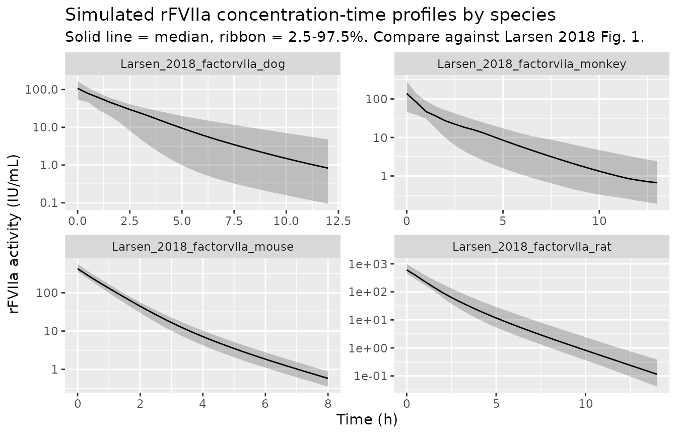
rFVIII: four-species simulation
sim_rfviii <- bind_rows(
  sim_species("Larsen_2018_factorviii_mouse",
              dose_IU  = 280 * 0.021,                # 280 IU/kg * 0.021 kg
              obs_grid = seq(0, 48, by = 1),
              n = 30L, id_offset =    0L,
              sexf = 0L,
              wt_range = c(0.019, 0.021)),
  sim_species("Larsen_2018_factorviii_rat",
              dose_IU  = 250 * 0.32,                 # 250 IU/kg * 0.32 kg
              obs_grid = seq(0, 24, by = 0.5),
              n = 30L, id_offset =  100L,
              sexf = 0L,
              wt_range = c(0.22, 0.41)),
  sim_species("Larsen_2018_factorviii_monkey",
              dose_IU  = 250 * 2.96,                 # 250 IU/kg * 2.96 kg
              obs_grid = seq(0, 48, by = 1),
              n = 30L, id_offset =  200L,
              wt_range = c(2.11, 3.97)),
  sim_species("Larsen_2018_factorviii_dog",
              dose_IU  = 100 * 19.55,                # 100 IU/kg * 19.55 kg
              obs_grid = seq(0, 80, by = 2),
              n = 30L, id_offset =  300L,
              wt_range = c(19.55, 19.8))
)
#> ℹ omega/sigma items treated as zero: 'etalvc', 'etalcl'
#> Warning: multi-subject simulation without without 'omega'
sim_rfviii |>
  group_by(label, time) |>
  summarise(
    lo  = quantile(Cc, 0.025, na.rm = TRUE),
    med = quantile(Cc, 0.50,  na.rm = TRUE),
    hi  = quantile(Cc, 0.975, na.rm = TRUE),
    .groups = "drop"
  ) |>
  ggplot(aes(time, med)) +
  geom_ribbon(aes(ymin = pmax(lo, 1e-3), ymax = hi), alpha = 0.25) +
  geom_line() +
  facet_wrap(~ label, scales = "free") +
  scale_y_log10() +
  labs(x = "Time (h)", y = "rFVIII activity (IU/mL)",
       title = "Simulated rFVIII concentration-time profiles by species",
       subtitle = "Solid line = median, ribbon = 2.5-97.5%. Compare against Larsen 2018 Fig. 2.")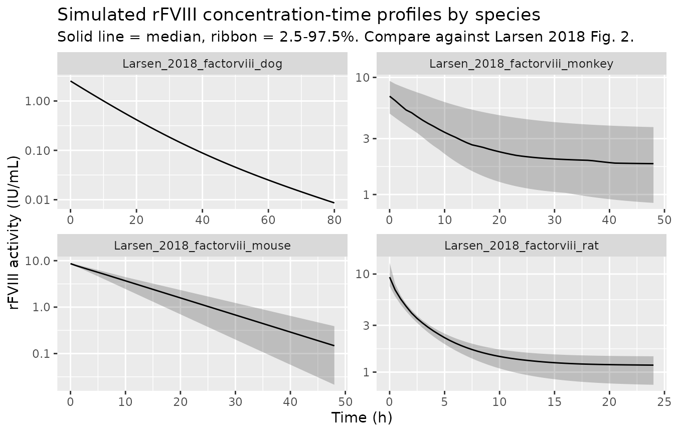
Nonlinear rFVIII clearance: rat dose sweep
The rat and monkey rFVIII models embed an exponential-nonlinear clearance (Larsen 2018 Eq. 1). To visualize the concentration dependence, we sweep the rat model across the three dose levels used in the paper (50, 250, 1250 IU/kg) at the median rat weight, zeroing IIV so the effect is deterministic.
mod_rat_fn <- readModelDb("Larsen_2018_factorviii_rat")
mod_rat    <- rxode2::zeroRe(mod_rat_fn())

dose_grid <- tibble(
  dose_iu_kg = c(50, 250, 1250),
  wt         = 0.32
) |>
  mutate(
    amt        = dose_iu_kg * wt,
    dose_label = sprintf("%d IU/kg", dose_iu_kg)
  )

ev_rat <- bind_rows(lapply(seq_len(nrow(dose_grid)), function(i) {
  d <- dose_grid[i, ]
  tibble(
    id    = i, time = 0, evid = 1L, amt = d$amt, cmt = "central",
    WT    = d$wt, SEXF = 0L,
    label = d$dose_label
  ) |>
    bind_rows(
      tibble(
        id    = i,
        time  = seq(0.05, 24, by = 0.25),
        evid  = 0L, amt = 0, cmt = "central",
        WT    = d$wt, SEXF = 0L,
        label = d$dose_label
      )
    )
}))

sim_rat_sweep <- rxode2::rxSolve(mod_rat, events = ev_rat, keep = c("label")) |>
  as.data.frame()
#> ℹ omega/sigma items treated as zero: 'etalrbase'
#> Warning: multi-subject simulation without without 'omega'

sim_rat_sweep |>
  ggplot(aes(time, Cc, colour = label)) +
  geom_line(linewidth = 0.9) +
  scale_y_log10() +
  labs(x = "Time (h)", y = "rFVIII activity (IU/mL)",
       colour = "Rat dose",
       title = "Rat rFVIII typical-value profiles by dose",
       subtitle = "Nonlinear CL rises with FVIII activity (Larsen 2018 Eq. 1)")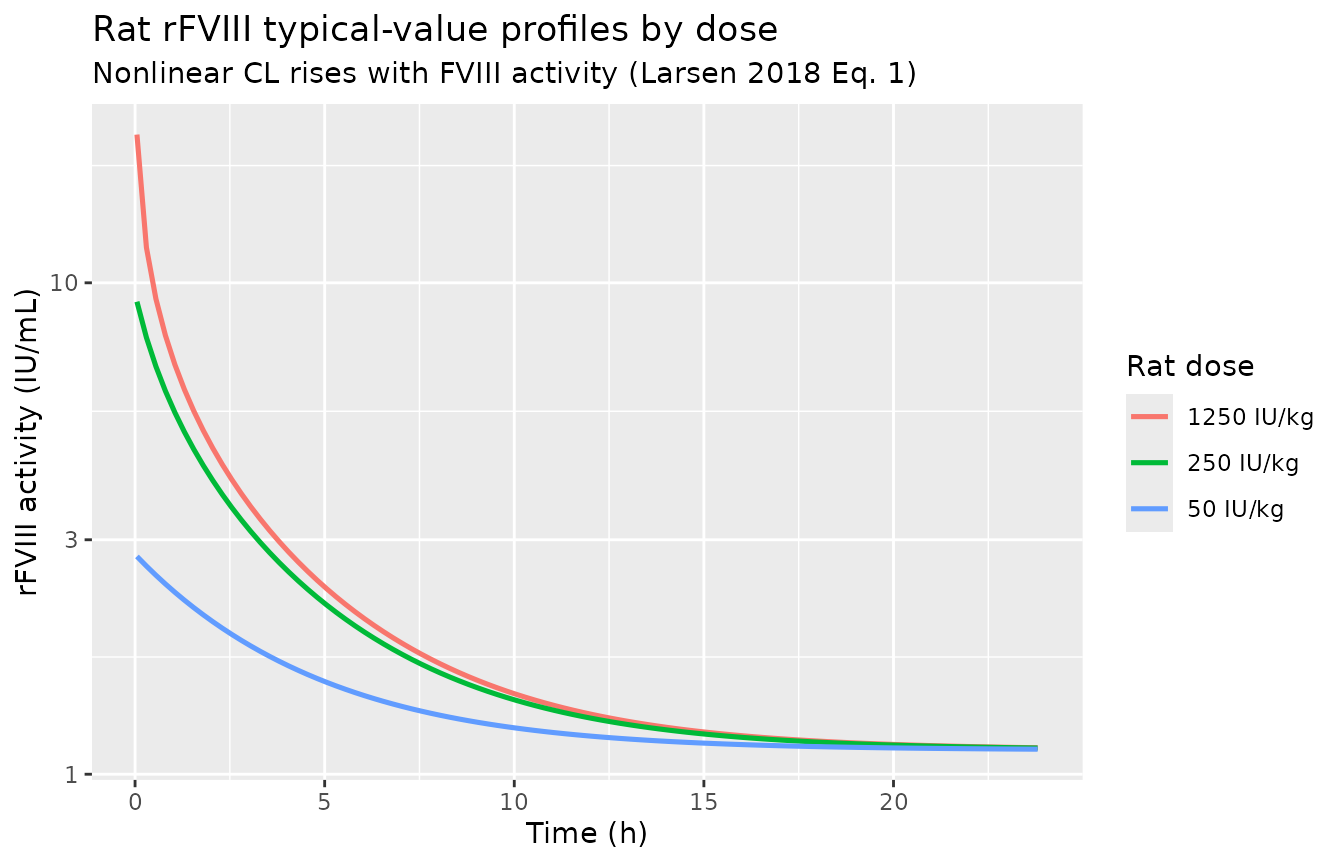
PKNCA validation
We run PKNCA on the monkey rFVIIa simulation (n = 30) as an illustrative NCA. The paper reports pcVPCs rather than an NCA table, so this section shows the simulated NCA parameters rather than a strict published-vs-simulated comparison.
sim_nca <- sim_rfviia |>
  filter(label == "Larsen_2018_factorviia_monkey", !is.na(Cc)) |>
  select(id, time, Cc, label)

# Guarantee a time=0 row per subject (endogenous baseline is 0 for the model's
# central compartment; monkey has an additive baseline captured via `rbase`,
# but the NCA baseline reference for AUC0-inf is total activity at t=0).
sim_nca <- bind_rows(
  sim_nca,
  sim_nca |> distinct(id, label) |> mutate(time = 0, Cc = 0.287)
) |>
  distinct(id, label, time, .keep_all = TRUE) |>
  arrange(id, label, time)

conc_obj <- PKNCA::PKNCAconc(sim_nca, Cc ~ time | label + id)

dose_df <- tibble(
  id    = unique(sim_nca$id),
  time  = 0,
  amt   = 270 * 2.78 * 50,        # 270 ug/kg * 2.78 kg * 50 IU/ug
  label = "Larsen_2018_factorviia_monkey"
)
dose_obj <- PKNCA::PKNCAdose(dose_df, amt ~ time | label + id)

intervals <- data.frame(
  start        = 0,
  end          = Inf,
  cmax         = TRUE,
  tmax         = TRUE,
  aucinf.obs   = TRUE,
  half.life    = TRUE
)

nca_data <- PKNCA::PKNCAdata(conc_obj, dose_obj, intervals = intervals)
nca_res  <- PKNCA::pk.nca(nca_data)

nca_summary <- as.data.frame(nca_res$result) |>
  filter(PPTESTCD %in% c("cmax", "tmax", "aucinf.obs", "half.life")) |>
  group_by(PPTESTCD) |>
  summarise(median = median(PPORRES, na.rm = TRUE),
            q05    = quantile(PPORRES, 0.05, na.rm = TRUE),
            q95    = quantile(PPORRES, 0.95, na.rm = TRUE),
            .groups = "drop")

nca_summary |>
  dplyr::rename(
    "NCA parameter"        = PPTESTCD,
    "Median"               = median,
    "5th percentile"       = q05,
    "95th percentile"      = q95
  ) |>
  knitr::kable(caption = "Simulated NCA summary for monkey rFVIIa (270 ug/kg IV; n = 30). Median half-life aligns with the published 2-compartment concentration-time profile in Larsen 2018 Fig. 1c.",
digits = 3)| NCA parameter | Median | 5th percentile | 95th percentile |
|---|---|---|---|
| aucinf.obs | 201.714 | 128.774 | 309.186 |
| cmax | 138.107 | 52.771 | 264.316 |
| half.life | 3.217 | 2.435 | 19.396 |
| tmax | 0.000 | 0.000 | 0.000 |
Assumptions and deviations
- Mass-to-activity conversion for rFVIIa – the paper reports rFVIIa doses in mass (ug/kg), while its Table 2 parameters are activity-scaled (IU/mL). For simulation, this vignette assumes 50 IU/ug specific activity (typical for eptacog alfa); users simulating a specific rFVIIa product must adjust the conversion to match the product-specific specific activity.
-
Endogenous baseline as an additive constant – the
monkey rFVIIa (0.287 IU/mL), rat rFVIII (1.12 IU/mL), and monkey rFVIII
(1.75 IU/mL) endogenous baselines are encoded as additive constants on
the observation
Cc = central/vc + rbase, with the central compartment holding only the dosed drug. This matches the paper’s typical NONMEM implementation and is exact when endogenous production balances endogenous elimination over the study window. The paper does not distinguish between an ODE-tracked steady-state pool and an additive baseline; the two are numerically indistinguishable at the observation grid for the reported half-lives. -
Nonlinear CL evaluated on total activity – for the
rat and monkey rFVIII models the exponential-nonlinear clearance
CL(C) = CL_0 * exp(beta * C)is evaluated on the total observed activity (central/vc + rbase). This is consistent with the paper’s mechanistic rationale (“supraphysiological concentrations … saturate von Willebrand factor binding sites, freeing more FVIII to clearance”) which relates to total, not just exogenous, FVIII. -
STRAIN_C57BI6 covariate – the mouse rFVIIa data
pool C57BI/6 and NMRI mice. The packaged model applies fractional strain
multipliers (V x 0.588, CL x 0.87 for C57BI/6 vs NMRI reference) when
STRAIN_C57BI6 = 1; the reference NMRI isSTRAIN_C57BI6 = 0. Users must supply the strain column in their event table (default reference NMRI is safe if unknown). -
Allometric scaling – the paper’s Sec 2.5 notes that
scaling principles I (theory-based, exponents 0.75 / 1) and II
(proportional, exponent 1 throughout) gave “insignificant” differences
within-species. This package encodes principle I; users wanting
principle II can override
e_wt_clande_wt_qat simulation time. - Weight range for dog rFVIII (n = 3) – the packaged parameters (particularly Q, RSE 83%) reflect a very small sample; the dog rFVIII model should be treated accordingly.
- No human popPK model is packaged – Larsen 2018 uses human data only for external validation and cites upstream human models (Bysted 2007 rFVIIa, Jimenez-Yuste 2015 rFVIII) rather than developing a new one. Users needing a human popPK model for rFVIIa or rFVIII should extract those upstream references separately.