Cefadroxil whole-body PBPK in mouse, rat and human (Tan 2021)

Model and source

• Citation: Tan Z, Zhang Y, Wang C, Sun L. Physiologically Based Pharmacokinetic Modeling of Cefadroxil in Mouse, Rat, and Human to Predict Concentration-Time Profile at Infected Tissue. Front Pharmacol. 2021;12:692741. doi:10.3389/fphar.2021.692741. PMCID PMC8733657. Tissue volumes and blood flows are Table 1 (mouse columns); partition coefficients are Table 3 (‘The K p values used in PBPK models’ column); the blood-to-plasma ratio, doses, renal clearance and Vss are Table 2; predicted AUC0-inf is Table 4; the predicted and observed profiles are Figure 3.
• Article: Front Pharmacol 2021;12:692741 (PMC8733657, open access).

Tan et al. built three whole-body physiologically based pharmacokinetic (PBPK) models of the cephalosporin cefadroxil in GastroPlus 9.7: a mouse and a rat model after an intravenous bolus, and a human model after oral dosing. All three share one structure: thirteen well-stirred, perfusion-rate-limited tissues between arterial and venous blood pools, with the spleen and gut draining into the liver through the portal vein. They also share one set of tissue-to-plasma partition coefficients (Kp). Each species has its own GastroPlus default physiology (Table 1) and its own renal clearance (Table 2). Elimination is renal only; over 90% of a dose is excreted unchanged in urine.

The paper prints every value the disposition layer needs except one, so the three models are packaged as three files:

File	Species	Dosing in the package
Tan_2021_cefadroxil_mouse_pbpk	mouse	IV bolus into venous (as in the paper)
Tan_2021_cefadroxil_rat_pbpk	rat	IV bolus into venous (as in the paper)
Tan_2021_cefadroxil_human_pbpk	human	absorbed dose into venous (disposition layer only; see Assumptions)

mods <- list(
  mouse = rxode2::rxode2(readModelDb("Tan_2021_cefadroxil_mouse_pbpk")),
  rat   = rxode2::rxode2(readModelDb("Tan_2021_cefadroxil_rat_pbpk")),
  human = rxode2::rxode2(readModelDb("Tan_2021_cefadroxil_human_pbpk"))
)

Population

None of the three models is a population fit. Each is a typical-value forward simulation of the GastroPlus default fasted physiology for its species. The renal clearance was optimised against the observed plasma profiles (Discussion, “Model Calibration”). The validation data were:

• Mouse: wild-type mice given 11, 44.5 and 528 nmol/g intravenously (0.1, 0.4 and 4.79 mg; Table 2). There were n = 6-8 per dose, sampled at 1-120 min (Posada and Smith 2013a; Hu and Smith 2016). Since 0.1 mg is 11 nmol/g at a molecular weight of 363.39 g/mol, the implied body weight is about 25 g.
• Rat: 2 mg/kg intravenously (0.62 mg, so about 0.31 kg), n = 4-5, femoral-artery samples at 0-240 min (Jin et al. 2014; Kim et al. 2014).
• Human: six healthy volunteers given 5 and 15 mg/kg orally, three of whom also received 30 mg/kg. The doses were 375.5, 1126.5 and 2253 mg, which implies about 75 kg (Garrigues et al. 1991).

The paper reports no between-subject variability and no residual-error model. All three files are therefore deterministic.

Source trace

Element	Value(s)	Source location
Model structure (13 perfusion-limited tissues, arterial / venous blood, portal drainage of gut and spleen)	–	Methods; Figures 1 and 2
Tissue volumes, per species (mL)	e.g. mouse lung 0.15833, rat muscle 151.28, human adipose 24307.3	Table 1, “Volume (ml)” columns
Tissue blood flows, per species (mL/s)	e.g. cardiac output 0.11347 / 0.9389 / 98.1779	Table 1, “The blood flow (ml/s)” columns
Total hepatic outflow q_liver = hepatic artery + gut + spleen	mouse 0.03352, rat 0.23111, human 24.3444	Table 1 row “Liver”; the flows balance against cardiac output only under this reading (checked below)
Gut (portal tributary) flow q_gut	0.02498 / 0.14689 / 12.263	Table 1 row “ACAT gut” (volume printed as “-”)
Kp, all tissues, all species	lung 0.52, adipose 0.1, muscle 0.25, liver 0.81, spleen 0.41, heart 0.23, brain 0.11, kidney 6.87, skin 0.89, reproductive organ 0.5, red marrow 0.47, yellow marrow 0.25, rest of body 0.5	Table 3, column “The K p values used in PBPK models”
Blood-to-plasma ratio bp	1	Table 2
Renal clearance cl_renal (L/h)	0.031 / 0.18 / 8.50	Table 2, “Clearance (L/h)”
Renal clearance acts on arterial plasma perfusing the kidney	–	Methods (“the kidney was designed as the elimination organ”); Limitations (“just the CL was added in the kidney”); confirmed by the human kidney:plasma Cmax ratio (below)
Plasma unbound fraction	71.9% (not used by the equations)	Table 2
Vss (L)	0.012 / 0.159 / 24.747 (Results text: 23.25 for human)	Table 2; Results
Predicted AUC0-inf (ug.h/mL)	mouse 3.17 / 12.69 / 151.98; rat 3.42; human 44.14 / 132.37 / 264.50	Table 4
Human predicted tissue Cmax after 15 mg/kg (ug/mL)	plasma 34.23, lung 17.8, adipose 3.4, muscle 8.33, liver 33.37, spleen 14.05, heart 7.88, brain 3.77, kidney 210.22, skin 29.79	Results, “The Physiologically Based Pharmacokinetic Models in Mouse, Rat, and Human”
Human fraction absorbed	99.9%	Results, “Effect of hPEPT1 on the Oral Absorption of Cefadroxil”
Predicted mouse and rat plasma profiles	–	Figures 3 and 4

Structural checks

Blood-flow balance

Cardiac output (the lung flow) must equal the sum of every flow returning to the venous blood: each non-splanchnic tissue plus the total hepatic outflow. The spleen and gut flows are already contained in the hepatic outflow.

flow_balance <- lapply(names(mods), function(sp) {
  th <- mods[[sp]]$theta
  q <- th[grepl("^q_", names(th))]
  returning <- q[setdiff(names(q), c("q_lung", "q_gut", "q_spleen"))]
  data.frame(
    species = sp,
    cardiac_output = q[["q_lung"]],
    sum_of_returning_flows = sum(returning),
    hepatic_artery = q[["q_liver"]] - q[["q_gut"]] - q[["q_spleen"]]
  )
}) |> bind_rows()
knitr::kable(flow_balance, digits = 5)

species	cardiac_output	sum_of_returning_flows	hepatic_artery
mouse	0.11347	0.11347	0.00704
rat	0.93890	0.93889	0.07247
human	98.17790	98.17797	9.24846

stopifnot(
  # Table 1 flows are printed to 5-6 significant figures.
  all(abs(flow_balance$sum_of_returning_flows / flow_balance$cardiac_output - 1) < 1e-4),
  all(flow_balance$hepatic_artery > 0)
)

The balance is exact to the printed precision in all three species. This confirms that Table 1’s liver flow is the total hepatic outflow and not the hepatic-artery flow.

Steady-state volume of distribution

For a perfusion-limited model with bp = 1, Vss is the blood volume plus the Kp-weighted sum of the tissue volumes.

vss <- lapply(names(mods), function(sp) {
  th <- mods[[sp]]$theta
  v <- th[grepl("^v_", names(th))] / 1000
  tis <- sub("^v_", "", names(v))
  kp <- ifelse(tis %in% c("arterial", "venous"), 1, exp(th[paste0("lkp_", tis)]))
  data.frame(species = sp, Vss_model_L = sum(v * kp))
}) |> bind_rows() |>
  mutate(Vss_Table2_L = c(0.012, 0.159, 24.747), pct_diff = 100 * (Vss_model_L / Vss_Table2_L - 1))
knitr::kable(vss, digits = 4)

species	Vss_model_L	Vss_Table2_L	pct_diff
mouse	0.0128	0.012	6.8752
rat	0.1673	0.159	5.1939
human	25.0047	24.747	1.0414

stopifnot(all(abs(vss$pct_diff) < 10))

The packaged models are 1-7% above the Table 2 Vss values. The human Results text gives yet another value (23.25 L) for the same quantity. The paper does not print the formula GastroPlus used for Vss, so the gap is reported here and not adjusted.

Replicating Figures 3 and 4 (mouse and rat intravenous bolus)

The predicted lines of Figures 3 and 4 were digitised by the maintainers from the published raster images. The y axis is logarithmic, so expect a few percent of reading error.

fig_pred <- tribble(
  ~species, ~dose_mg, ~time, ~pred_paper,
  "mouse", 0.1, 0.6, 1.6681, "mouse", 0.1, 0.9, 0.837, "mouse", 0.1, 1.1, 0.5364,
  "mouse", 0.1, 1.3, 0.3437, "mouse", 0.1, 1.65, 0.1613, "mouse", 0.1, 1.85, 0.1069,
  "mouse", 0.4, 0.6, 6.6261, "mouse", 0.4, 0.9, 3.3246, "mouse", 0.4, 1.1, 2.1785,
  "mouse", 0.4, 1.3, 1.3807, "mouse", 0.4, 1.65, 0.6553, "mouse", 0.4, 1.85, 0.4246,
  "mouse", 4.79, 0.6, 77.4264, "mouse", 4.79, 0.9, 39.7222, "mouse", 4.79, 1.1, 25.4564,
  "mouse", 4.79, 1.3, 16.314, "mouse", 4.79, 1.65, 7.657, "mouse", 4.79, 1.85, 5.0175,
  "rat", 0.62, 0.1, 3.3174, "rat", 0.62, 0.25, 2.6494, "rat", 0.62, 0.5, 1.9795,
  "rat", 0.62, 0.75, 1.5291, "rat", 0.62, 1, 1.1521, "rat", 0.62, 1.5, 0.6761,
  "rat", 0.62, 2, 0.3968, "rat", 0.62, 2.5, 0.2329, "rat", 0.62, 3, 0.1367,
  "rat", 0.62, 3.5, 0.0815, "rat", 0.62, 3.98, 0.0503
)

grid <- sort(unique(c(seq(0, 0.1, by = 0.002), seq(0.1, 4, by = 0.01), seq(4, 48, by = 0.1),
                      fig_pred$time)))
sim_one <- function(species, dose_mg, times = grid) {
  ev <- rxode2::et(amt = dose_mg, cmt = "venous") |> rxode2::et(times)
  as.data.frame(rxode2::rxSolve(mods[[species]], events = ev, rtol = 1e-10, atol = 1e-12)) |>
    mutate(species = species, dose_mg = dose_mg)
}
iv_doses <- tribble(~species, ~dose_mg, "mouse", 0.1, "mouse", 0.4, "mouse", 4.79, "rat", 0.62)
sim_iv <- bind_rows(Map(sim_one, iv_doses$species, iv_doses$dose_mg))

sim_iv |>
  filter(time > 0, time <= 4) |>
  mutate(group = paste(species, dose_mg, "mg")) |>
  ggplot(aes(time, Cc, colour = group)) +
  geom_line() +
  geom_point(data = mutate(fig_pred, group = paste(species, dose_mg, "mg")), aes(y = pred_paper)) +
  scale_y_log10() +
  facet_wrap(~species, scales = "free") +
  labs(x = "Time (h)", y = "Plasma cefadroxil (mg/L)", colour = NULL)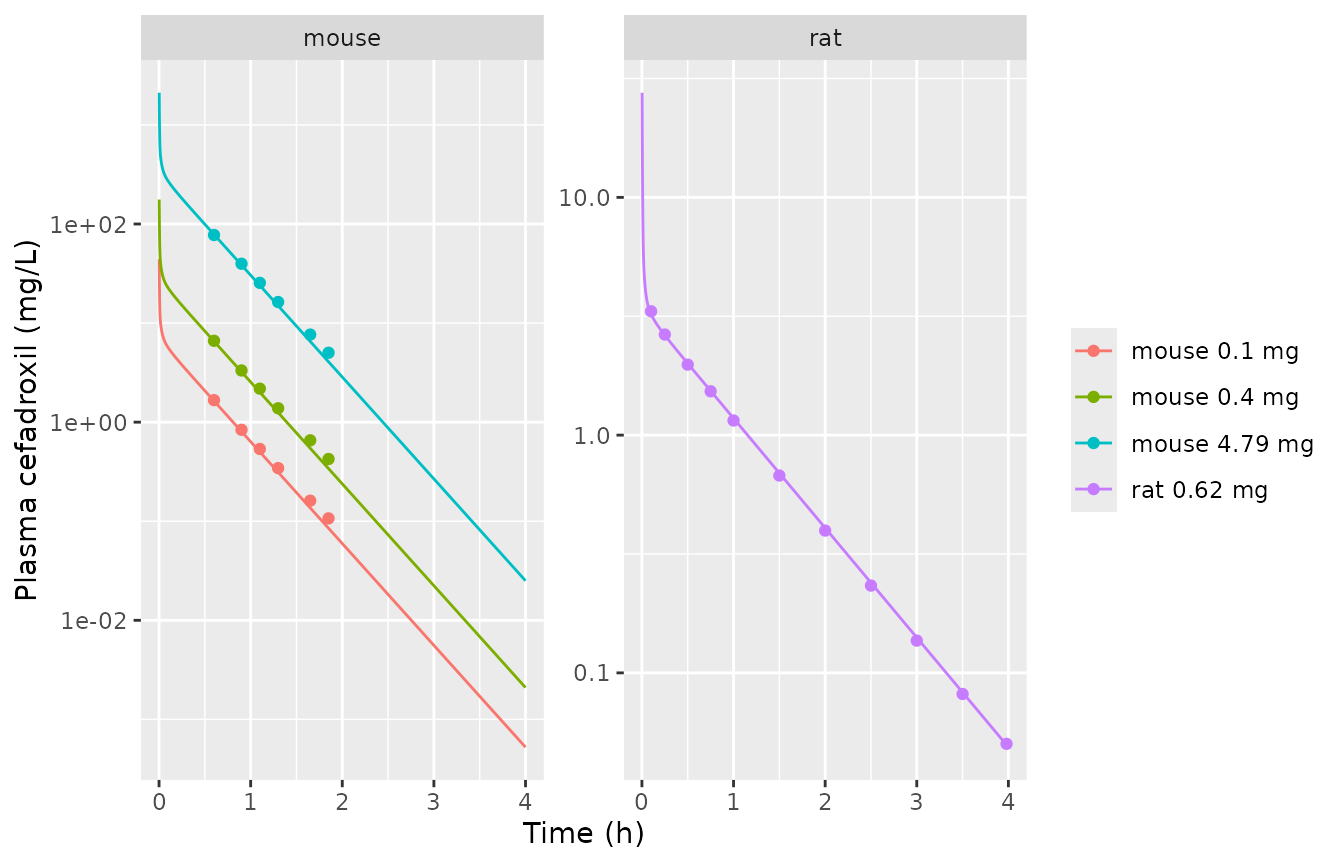

Replicates the predicted lines of Figures 3 (mouse) and 4 (rat) of Tan 2021. Lines: packaged models. Points: the paper’s predicted lines, digitised.

fig_cmp <- fig_pred |>
  inner_join(select(sim_iv, species, dose_mg, time, Cc), by = c("species", "dose_mg", "time")) |>
  mutate(pct_diff = 100 * (Cc / pred_paper - 1))
stopifnot(nrow(fig_cmp) == nrow(fig_pred))
fig_cmp |>
  rename("Species" = species, "Dose (mg)" = dose_mg, "Time (h)" = time,
         "Paper (digitised)" = pred_paper, "Package" = Cc, "% diff" = pct_diff) |>
  knitr::kable(digits = c(0, 2, 2, 4, 4, 1))

Species	Dose (mg)	Time (h)	Paper (digitised)	Package	% diff
mouse	0.10	0.60	1.6681	1.6369	-1.9
mouse	0.10	0.90	0.8370	0.8047	-3.9
mouse	0.10	1.10	0.5364	0.5012	-6.6
mouse	0.10	1.30	0.3437	0.3122	-9.2
mouse	0.10	1.65	0.1613	0.1364	-15.5
mouse	0.10	1.85	0.1069	0.0850	-20.5
mouse	0.40	0.60	6.6261	6.5475	-1.2
mouse	0.40	0.90	3.3246	3.2187	-3.2
mouse	0.40	1.10	2.1785	2.0050	-8.0
mouse	0.40	1.30	1.3807	1.2490	-9.5
mouse	0.40	1.65	0.6553	0.5455	-16.8
mouse	0.40	1.85	0.4246	0.3398	-20.0
mouse	4.79	0.60	77.4264	78.4064	1.3
mouse	4.79	0.90	39.7222	38.5436	-3.0
mouse	4.79	1.10	25.4564	24.0096	-5.7
mouse	4.79	1.30	16.3140	14.9562	-8.3
mouse	4.79	1.65	7.6570	6.5325	-14.7
mouse	4.79	1.85	5.0175	4.0693	-18.9
rat	0.62	0.10	3.3174	3.2232	-2.8
rat	0.62	0.25	2.6494	2.6302	-0.7
rat	0.62	0.50	1.9795	2.0023	1.2
rat	0.62	0.75	1.5291	1.5347	0.4
rat	0.62	1.00	1.1521	1.1769	2.2
rat	0.62	1.50	0.6761	0.6921	2.4
rat	0.62	2.00	0.3968	0.4070	2.6
rat	0.62	2.50	0.2329	0.2394	2.8
rat	0.62	3.00	0.1367	0.1408	3.0
rat	0.62	3.50	0.0815	0.0828	1.6
rat	0.62	3.98	0.0503	0.0497	-1.1

rat_cmp <- filter(fig_cmp, species == "rat")
mouse_cmp <- filter(fig_cmp, species == "mouse")
stopifnot(
  # Rat: the whole Figure 4 line reproduces within reading error.
  all(abs(rat_cmp$pct_diff) < 5),
  # Mouse: the early distribution phase reproduces ...
  all(abs(mouse_cmp$pct_diff[mouse_cmp$time == 0.6]) < 5),
  # ... and the late tail runs low (see Assumptions: the unprinted gut tissue).
  all(abs(mouse_cmp$pct_diff) < 25)
)

The rat line reproduces within 3% at every digitised time. The mouse lines agree within 2% at 0.6 h. After that the packaged model falls steadily lower than the paper, reaching about 20% low by 1.85 h. This is the same for all three doses because the model is linear. The terminal slope of the packaged mouse model is about 2.37 /h, against about 2.19 /h in Figure 3. The paper’s mouse model therefore holds slightly more drug outside the plasma. The likely source is the GastroPlus gut tissue, whose volume and Kp the paper does not print (see Assumptions).

PKNCA validation against Table 4

Both the human model in this package and the mouse and rat models are dosed as an intravenous bolus. Table 4’s human Cmax values come from oral absorption, so only AUC0-inf is compared. For the human, the three Table 4 doses are simulated as the absorbed amount.

human_doses <- c(375.5, 1126.5, 2253)
sim_all <- bind_rows(sim_iv, bind_rows(lapply(human_doses, function(d) sim_one("human", d)))) |>
  mutate(treatment = paste(species, dose_mg, "mg"), id = 1L)
stopifnot(all(sim_all$Cc >= -1e-6 * max(sim_all$Cc)))
conc_df <- sim_all |>
  filter(!is.na(Cc)) |>
  mutate(Cc = pmax(Cc, 0)) |>
  group_by(treatment) |>
  filter(time <= time[which.max(Cc)] | Cc >= 1e-6 * max(Cc)) |>
  ungroup() |>
  select(id, treatment, time, Cc)
dose_df <- distinct(sim_all, id, treatment, dose_mg) |> mutate(time = 0)
o_conc <- PKNCA::PKNCAconc(conc_df, Cc ~ time | treatment + id)
o_dose <- PKNCA::PKNCAdose(dose_df, dose_mg ~ time | treatment + id, route = "intravascular")
o_data <- PKNCA::PKNCAdata(o_conc, o_dose,
  intervals = data.frame(start = 0, end = Inf, aucinf.obs = TRUE, cmax = TRUE, half.life = TRUE))
nca <- PKNCA::pk.nca(o_data)

reference <- data.frame(
  treatment = c("mouse 0.1 mg", "mouse 0.4 mg", "mouse 4.79 mg", "rat 0.62 mg",
                "human 375.5 mg", "human 1126.5 mg", "human 2253 mg"),
  aucinf.obs = c(3.17, 12.69, 151.98, 3.42, 44.14, 132.37, 264.50)
)
cmp <- nlmixr2lib::ncaComparisonTable(nca, reference, by = "treatment",
  params = "aucinf.obs", units = c(aucinf.obs = "mg*h/L"))
knitr::kable(cmp)

NCA parameter	treatment	Reference	Simulated	% diff
AUC0-∞ (obs) (mg*h/L)	mouse 0.1 mg	3.17	3.23	+1.9%
AUC0-∞ (obs) (mg*h/L)	mouse 0.4 mg	12.7	12.9	+1.8%
AUC0-∞ (obs) (mg*h/L)	mouse 4.79 mg	152	155	+1.8%
AUC0-∞ (obs) (mg*h/L)	rat 0.62 mg	3.42	3.44	+0.7%
AUC0-∞ (obs) (mg*h/L)	human 375.5 mg	44.1	44.2	+0.1%
AUC0-∞ (obs) (mg*h/L)	human 1126.5 mg	132	133	+0.1%
AUC0-∞ (obs) (mg*h/L)	human 2253 mg	264	265	+0.2%

auc <- as.data.frame(nca) |>
  filter(PPTESTCD == "aucinf.obs") |>
  left_join(reference, by = "treatment") |>
  left_join(distinct(sim_all, treatment, species, dose_mg), by = "treatment") |>
  mutate(
    cl = c(mouse = 0.031, rat = 0.18, human = 8.50)[species],
    dose_over_cl = dose_mg / cl,
    pct_vs_table4 = 100 * (PPORRES / aucinf.obs - 1)
  )
stopifnot(
  nrow(auc) == 7,
  # A clearance acting on arterial plasma gives AUC = Dose / CL exactly;
  # the residual is trapezoid error on a fine grid.
  all(abs(auc$PPORRES / auc$dose_over_cl - 1) < 0.005),
  # Table 4 is reproduced within 2% (mouse 0.031 L/h is a rounded value).
  all(abs(auc$pct_vs_table4) < 2.5)
)

Every AUC0-inf is within 2% of Table 4, and for each species and dose AUC0-inf equals Dose / CL. The three mouse AUCs in Table 4 are all 1.8% below Dose / CL. They imply a clearance of about 0.0315 L/h, which is consistent with the printed 0.031 L/h being rounded. The Limitations section gives 0.52 mL/min, which is 0.0312 L/h. If the clearance acted on the venous outflow of the kidney, the AUC would be (Dose / CL)(1 + CL / Q_kidney) instead. For the rat that is about 4.4, which Table 4 rules out.

Human tissue distribution

The Results text gives the predicted human tissue Cmax after 15 mg/kg orally. For a perfusion-limited tissue without elimination, the tissue:plasma AUC ratio equals Kp exactly. For the kidney, which carries the renal clearance on its arterial inflow, it equals Kp (1 - CL / Q_kidney). Near Tmax the paper’s tissue:plasma Cmax ratios should approach these values.

h <- filter(sim_all, treatment == "human 1126.5 mg")
trap <- function(x, y) sum(diff(x) * (head(y, -1) + tail(y, -1)) / 2)
paper_cmax <- c(lung = 17.8, adipose = 3.4, muscle = 8.33, liver = 33.37, spleen = 14.05,
                heart = 7.88, brain = 3.77, kidney = 210.22, skin = 29.79)
tissue <- data.frame(tissue = names(paper_cmax)) |>
  mutate(
    model_auc_ratio = vapply(tissue, function(t) trap(h$time, h[[paste0("c_", t)]]) / trap(h$time, h$Cc), numeric(1)),
    paper_cmax_ratio = paper_cmax[tissue] / 34.23,
    pct_diff = 100 * (model_auc_ratio / paper_cmax_ratio - 1)
  )
knitr::kable(tissue, digits = 3)

tissue	model_auc_ratio	paper_cmax_ratio	pct_diff
lung	0.520	0.520	-0.046
adipose	0.100	0.099	0.670
muscle	0.250	0.243	2.724
liver	0.810	0.975	-16.917
spleen	0.410	0.410	-0.117
heart	0.230	0.230	-0.095
brain	0.110	0.110	-0.130
kidney	6.136	6.141	-0.090
skin	0.890	0.870	2.258

th_h <- mods$human$theta
kid_expected <- exp(th_h[["lkp_kidney"]]) * (1 - exp(th_h[["lcl_renal"]]) / (th_h[["q_kidney"]] * 3.6))
stopifnot(
  abs(tissue$model_auc_ratio[tissue$tissue == "kidney"] / kid_expected - 1) < 1e-3,
  # Every tissue except the liver: the paper's oral Cmax ratios match the
  # model's equilibrium ratios (the liver sees the absorbed dose first).
  all(abs(tissue$pct_diff[tissue$tissue != "liver"]) < 5)
)

All tissues except the liver agree within 3%. The kidney ratio of 6.14 matches the paper’s 210.22 / 34.23 = 6.14. This confirms that renal clearance is taken from the arterial plasma entering the kidney and that Kp is relative to total plasma. The paper’s liver ratio (0.97) is above Kp (0.81) because, after oral dosing, the absorbed drug passes through the liver on the way to systemic blood. The disposition-only model does not include that first pass.

h |>
  filter(time > 0, time <= 12) |>
  select(time, plasma = Cc, kidney = c_kidney, liver = c_liver, skin = c_skin,
         lung = c_lung, muscle = c_muscle, brain = c_brain) |>
  pivot_longer(-time, names_to = "tissue", values_to = "conc") |>
  ggplot(aes(time, conc, colour = tissue)) +
  geom_line() +
  scale_y_log10() +
  labs(x = "Time (h)", y = "Cefadroxil (mg/L)", colour = NULL)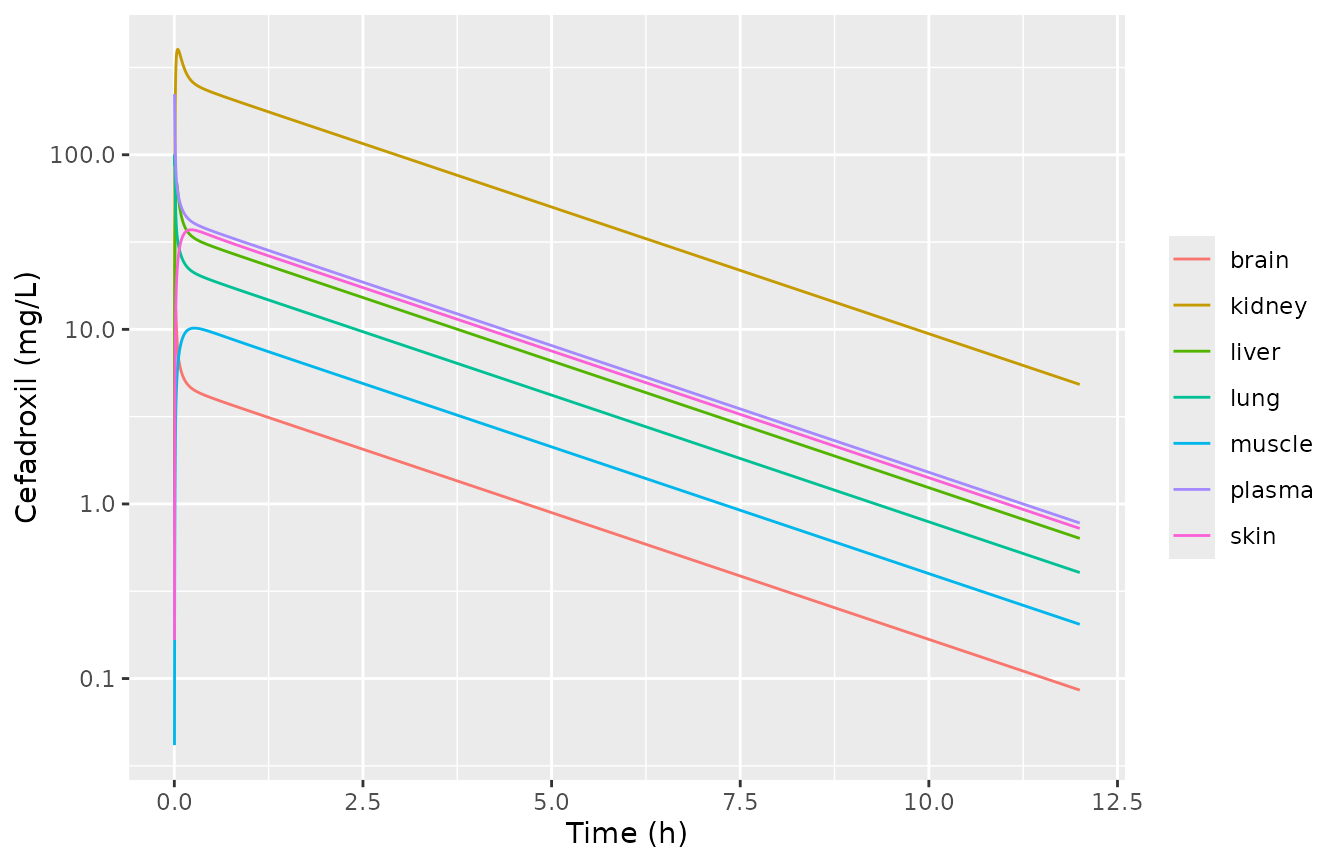

Human plasma and tissue concentrations after 1126.5 mg (15 mg/kg) absorbed into venous blood. Compare with Supplementary Figure S1 of Tan 2021, which shows the oral profile.

Assumptions and deviations

• ACAT gut tissue (all species). Table 1 gives a blood flow for the GastroPlus “ACAT gut” tissue but prints its volume as “-”, and Table 3 has no gut Kp. That tissue belongs to GastroPlus’s internal enterocyte physiology and is not published. In the package it is a zero-volume pass-through: its portal flow reaches the liver at the arterial concentration. This adds no unpublished constant. The rat profile and every AUC reproduce. The mouse terminal phase is somewhat steeper than Figure 3. That is consistent with a missing gut distribution volume of roughly 1 mL in the mouse, but that volume was not back-solved from the figure. The maintainers chose this encoding over deferring the paper for author correspondence.
• Human oral absorption is not reproduced. The paper uses the GastroPlus ACAT model with hPEPT1-mediated uptake: hPEPT1 Km 860.31 mg/L, Vmax 0.0025 ug/s/mg hPEPT1, and 16.28-87.84 mg hPEPT1 per segment. The ACAT segment volumes, transit times and absorption scale factors are not printed, so the absorption time course cannot be rebuilt. The human file is the disposition layer, and a dose enters the venous blood directly. Human Cmax values from this file are therefore intravenous-bolus values. They are not comparable to Table 4’s oral Cmax and are not compared. Because the paper’s fraction absorbed is 99.9%, AUC is preserved.
• Plasma concentration. Cc is the venous plasma concentration, the GastroPlus “plasma” output. Rat samples were drawn from the femoral artery. Arterial and venous AUCs are identical, and the two profiles differ only in the first minutes. The arterial concentration is available as c_arterial.
• Unbound fraction. The plasma unbound fraction (71.9%) is listed in Table 2 but does not enter the equations: the Kp values and the renal clearance are both relative to total plasma. The tissue-ratio check above confirms this.
• Vss. The packaged models’ Vss is 1-7% above Table 2 (see above). The paper does not state how GastroPlus computes the tabulated value.
• New compartment names. reproductive_organ, red_marrow and yellow_marrow were registered for the GastroPlus “ReproOrg”, “Red marrow” and “Yellow marrow” tissues. bonemarrow stays the name for a single undivided marrow pool. testes was not used because the GastroPlus reproductive organ is not specified by sex.
• Supplement. Supplementary Figures S1-S2 and Table S1 (human tissue profiles and dissolution-rate sensitivity) were not used. The tissue Cmax values needed for the check above are given in the Results text.
• No variability. The paper reports no between-subject variability or residual error. The models are typical-value only.