Clofazimine (Stemkens 2024)
Source:vignettes/articles/Stemkens_2024_clofazimine.Rmd
Stemkens_2024_clofazimine.RmdModel and source
- Citation: Stemkens R, Lemson A, Koele SE, Svensson EM, te Brake LHM, van Crevel R, Boeree MJ, Hoefsloot W, van Ingen J, Aarnoutse RE (2024). A loading dose of clofazimine to rapidly achieve steady-state-like concentrations in patients with nontuberculous mycobacterial disease. J Antimicrob Chemother 79(12):3100-3108. doi:10.1093/jac/dkae309
- Description: Two-compartment population PK model for oral clofazimine in adults with pulmonary or extrapulmonary nontuberculous mycobacterial (NTM) disease, fitted to the pooled C-LOAD loading-dose study (300 mg once daily for 4 weeks, then 100 mg once daily) and the PERC trial (100 mg once daily, no loading dose). Absorption runs through a depot and one transit compartment that share a single rate constant (0.683 1/h). Apparent clearance (4.17 L/h), central volume (460 L), intercompartmental clearance (24.6 L/h) and peripheral volume (10100 L) are allometrically scaled on total body weight (70 kg reference; fixed exponents 0.75 for clearances and 1 for volumes). Relative bioavailability of each 300 mg dose is 0.736 times that of a 100 mg dose. Random effects are between-subject variability on clearance and on the absorption rate constant and inter-occasion variability on bioavailability of the doses given on PK sampling days; residual error is combined proportional plus additive.
- Article: https://doi.org/10.1093/jac/dkae309 (open access, PMC11638672)
- Supplement: Supplementary data at JAC Online (Text S3 holds the final NONMEM control stream)
Clofazimine has a very large volume of distribution and a terminal half-life of months, so plasma concentrations take most of a year to approach steady state at the standard 100 mg once-daily dose. Stemkens et al. studied a 4-week 300 mg once-daily loading phase (the C-LOAD study), pooled the data with the PERC trial (100 mg once daily without loading), and used the resulting population PK model to simulate alternative loading regimens.
Population
C-LOAD enrolled 12 adults with pulmonary (9) or extrapulmonary (3) nontuberculous mycobacterial (NTM) disease at Radboud University Medical Center, Nijmegen, the Netherlands: median age 69 years (range 39-82), median body weight 62 kg (51-105), median fat-free mass 50 kg (38-70), 50% male, 10 Caucasian and 2 Middle Eastern participants (Table 1). Most had M. avium complex disease and all received other antimycobacterial drugs (azithromycin in 11, ethambutol in 9, intravenous amikacin in 8, rifampicin in 7). The 19 PERC participants had M. avium complex pulmonary disease and received 100 mg once daily; their demographics are not tabulated in this paper. The model was fitted to 112 C-LOAD and 67 PERC concentrations.
The same information is available programmatically via
readModelDb("Stemkens_2024_clofazimine")()$population.
Source trace
Every ini() value carries an in-file comment pointing to
its source. Table 4 of the paper and the Text S3 control stream agree on
all fixed effects; the table below collects them.
| Equation / parameter | Value | Source location |
|---|---|---|
lcl (CL/F, 70 kg) |
log(4.17 L/h) | Table 4; Text S3 THETA(1) |
lvc (V/F, 70 kg) |
log(460 L) | Table 4; Text S3 THETA(2) |
lka (absorption and transit rate) |
log(0.683 1/h) | Table 4; Text S3 THETA(3), used for K12 and K23 |
lq (Q/F, 70 kg) |
log(24.6 L/h) | Table 4; Text S3 THETA(4) |
lvp (Vp/F, 70 kg) |
log(10100 L) | Table 4; Text S3 THETA(5) |
lfdepot |
log(1), fixed | Text S3 F1 = 1*IOVF*highdoseEFF
|
e_dose_high_fdepot |
0.736 | Table 4 ‘Effect of high-dose on bioavailability’ 73.6%; Text S3 THETA(6) |
e_wt_cl, e_wt_vc
|
0.75, 1 (fixed) | Table 4 footnote b; Text S3 AlloCL,
AlloV
|
etalcl |
0.55 | Text S3 $OMEGA; Table 4 IIV CL 85.6% CV |
etalka |
0.501 | Text S3 $OMEGA; Table 4 IIV absorption-rate constant 80.6% CV |
etaiov_fdepot_1..3 |
0.488 (2 and 3 fixed equal) | Text S3 $OMEGA BLOCK(1) + 2 x SAME; Table 4 IOV F 79.3% CV |
propSd |
0.08 | Table 4 ‘Proportional error’ 8.00%; Text S3 $SIGMA 0.00639 |
addSd |
0.0417 mg/L | Text S3 $SIGMA 0.00174 (variance); see Assumptions |
| Allometric scaling |
(WT/70)^0.75 on CL, Q; (WT/70)^1 on V,
Vp |
Text S3 $PK |
| ODEs | depot -> transit1 -> central <-> peripheral1, both
absorption steps at ka
|
Text S3 $MODEL / ADVAN5 rate constants; Figure S1 |
f(depot) |
exp(lfdepot + iov) * 0.736^DOSE_HIGH |
Text S3 $PK |
| Residual error | Cc * (1 + eps1) + eps2 |
Text S3 $ERROR |
The CV% values of Table 4 are reproduced from the control-stream variances with the paper’s own formula (footnote c, CV = sqrt(exp(omega) - 1)):
omega <- c(etalcl = 0.55, etalka = 0.501, etaiov_fdepot = 0.488)
cv_model <- round(100 * sqrt(exp(omega) - 1), 1)
cv_table4 <- c(etalcl = 85.6, etalka = 80.6, etaiov_fdepot = 79.3)
knitr::kable(data.frame(
  random_effect = names(omega), variance = omega,
  cv_from_variance = cv_model, cv_table4 = cv_table4
), row.names = FALSE)| random_effect | variance | cv_from_variance | cv_table4 |
|---|---|---|---|
| etalcl | 0.550 | 85.6 | 85.6 |
| etalka | 0.501 | 80.6 | 80.6 |
| etaiov_fdepot | 0.488 | 79.3 | 79.3 |
Model structure check: terminal half-life
The paper’s Discussion quotes a terminal half-life of about 80 days. The typical-value micro-constants of the packaged model (70 kg) give:
mod <- readModelDb("Stemkens_2024_clofazimine")
ui <- rxode2::rxode(mod)
#> ℹ parameter labels from comments will be replaced by 'label()'
#> Warning: some etas defaulted to non-mu referenced, possible parsing error: etaiov_fdepot_1, etaiov_fdepot_2, etaiov_fdepot_3
#> as a work-around try putting the mu-referenced expression on a simple line
th <- exp(ui$theta[c("lcl", "lvc", "lq", "lvp")])
k10 <- th[["lcl"]] / th[["lvc"]]
k12 <- th[["lq"]] / th[["lvc"]]
k21 <- th[["lq"]] / th[["lvp"]]
s <- k10 + k12 + k21
beta <- (s - sqrt(s^2 - 4 * k10 * k21)) / 2
thalf_days <- log(2) / beta / 24
thalf_days
#> [1] 84.54872
stopifnot(thalf_days > 70, thalf_days < 95)
Solver settings
A daily oral dose over most of a year combined with a sharp
absorption peak and an 85-day terminal phase exhausts LSODA’s default
step budget (“could not solve the system”). Every long simulation below
caps the step at 4 h and raises the step limit; steady-state
(ss = 1) solves also raise maxSS, because the
slow phase needs many dosing intervals to converge.
solve_long <- function(model, events, ...) {
  rxode2::rxSolve(
    model,
    events = events,
    hmax = 4,
    maxsteps = 1e6,
    maxSS = 20000,
    returnType = "data.frame",
    ...
  )
}
Replicate Figure 3: typical-patient trough profiles
Figure 3 shows simulated trough (pre-dose) concentrations for a
typical 65 kg patient on three regimens, with a dashed target line at
80% of the “predicted steady-state trough”. Inter-occasion variability
is switched off by setting OCC = 0 on every record, and the
doses are labelled with DOSE_HIGH (1 for 300 mg, 0 for 100
mg).
horizon_days <- 336 # 48 weeks, the end of the Figure 3 time axis (about 11 months)

make_regimen <- function(id, loading_dose, loading_weeks, wt, regimen,
                         ndays = horizon_days) {
  day <- 0:ndays
  dose_day <- day[day < ndays]
  amt <- ifelse(dose_day < loading_weeks * 7, loading_dose, 100)
  doses <- tibble(
    id = id, time = dose_day * 24, evid = 1L, amt = amt, cmt = "depot",
    DOSE_HIGH = as.integer(amt == 300)
  )
  # One trough record per day, placed BEFORE that day's dose (evid 0 sorts
  # first at a shared time), so the value is the pre-dose concentration.
  troughs <- tibble(
    id = id, time = day * 24, evid = 0L, amt = NA_real_, cmt = "central",
    DOSE_HIGH = NA_integer_
  )
  bind_rows(troughs, doses) |>
    arrange(id, time, evid) |>
    tidyr::fill(DOSE_HIGH, .direction = "up") |>
    mutate(DOSE_HIGH = tidyr::replace_na(DOSE_HIGH, 0L), WT = wt, OCC = 0L,
           regimen = regimen)
}

regimens <- tibble(
  regimen = c("100 mg once daily", "300 mg once daily 4 weeks",
              "300 mg once daily 6 weeks", "300 mg once daily 8 weeks"),
  loading_dose = c(100, 300, 300, 300),
  loading_weeks = c(0, 4, 6, 8)
)
mod_typical <- rxode2::zeroRe(mod)
#> ℹ parameter labels from comments will be replaced by 'label()'
#> Warning: some etas defaulted to non-mu referenced, possible parsing error: etaiov_fdepot_1, etaiov_fdepot_2, etaiov_fdepot_3
#> as a work-around try putting the mu-referenced expression on a simple line
#> Warning: some etas defaulted to non-mu referenced, possible parsing error: etaiov_fdepot_1, etaiov_fdepot_2, etaiov_fdepot_3
#> as a work-around try putting the mu-referenced expression on a simple line
ev_typical <- bind_rows(lapply(seq_len(nrow(regimens)), function(i) {
  make_regimen(i, regimens$loading_dose[i], regimens$loading_weeks[i],
               wt = 65, regimen = regimens$regimen[i])
}))
sim_typical <- solve_long(mod_typical, ev_typical, keep = "regimen") |>
  mutate(months = time / 24 / 30.4375)
#> ℹ omega/sigma items treated as zero: 'etalcl', 'etalka', 'etaiov_fdepot_1', 'etaiov_fdepot_2', 'etaiov_fdepot_3'
#> Warning: multi-subject simulation without without 'omega'

# True steady-state trough at 100 mg once daily (ss = 1), 65 kg.
ev_ss <- tibble(
  id = 1L, time = c(0, 24), evid = c(1L, 0L), amt = c(100, NA),
  ii = c(24, 0), ss = c(1L, 0L), cmt = c("depot", "central"),
  WT = 65, OCC = 0L, DOSE_HIGH = 0L
)
trough_ss_true <- solve_long(mod_typical, ev_ss)$Cc[1]
#> ℹ omega/sigma items treated as zero: 'etalcl', 'etalka', 'etaiov_fdepot_1', 'etaiov_fdepot_2', 'etaiov_fdepot_3'
trough_end <- sim_typical |>
  filter(regimen == "100 mg once daily", time == horizon_days * 24) |>
  pull(Cc)
target_typical <- 0.8 * trough_end
c(true_steady_state = trough_ss_true, end_of_horizon = trough_end,
  target = target_typical)
#> true_steady_state    end_of_horizon            target
#>         0.9819339         0.9270334         0.7416267

sim_typical |>
  filter(regimen != "300 mg once daily 8 weeks") |>
  ggplot(aes(months, Cc, colour = regimen, linetype = regimen)) +
  geom_line(linewidth = 1) +
  geom_hline(yintercept = target_typical, linetype = "dashed") +
  labs(
    x = "Time after start of treatment (months)",
    y = "Simulated clofazimine trough concentration (mg/L)",
    colour = "Loading dose regimen", linetype = "Loading dose regimen",
    caption = "Replicates Figure 3 of Stemkens 2024 (typical 65 kg patient)."
  ) +
  theme_bw()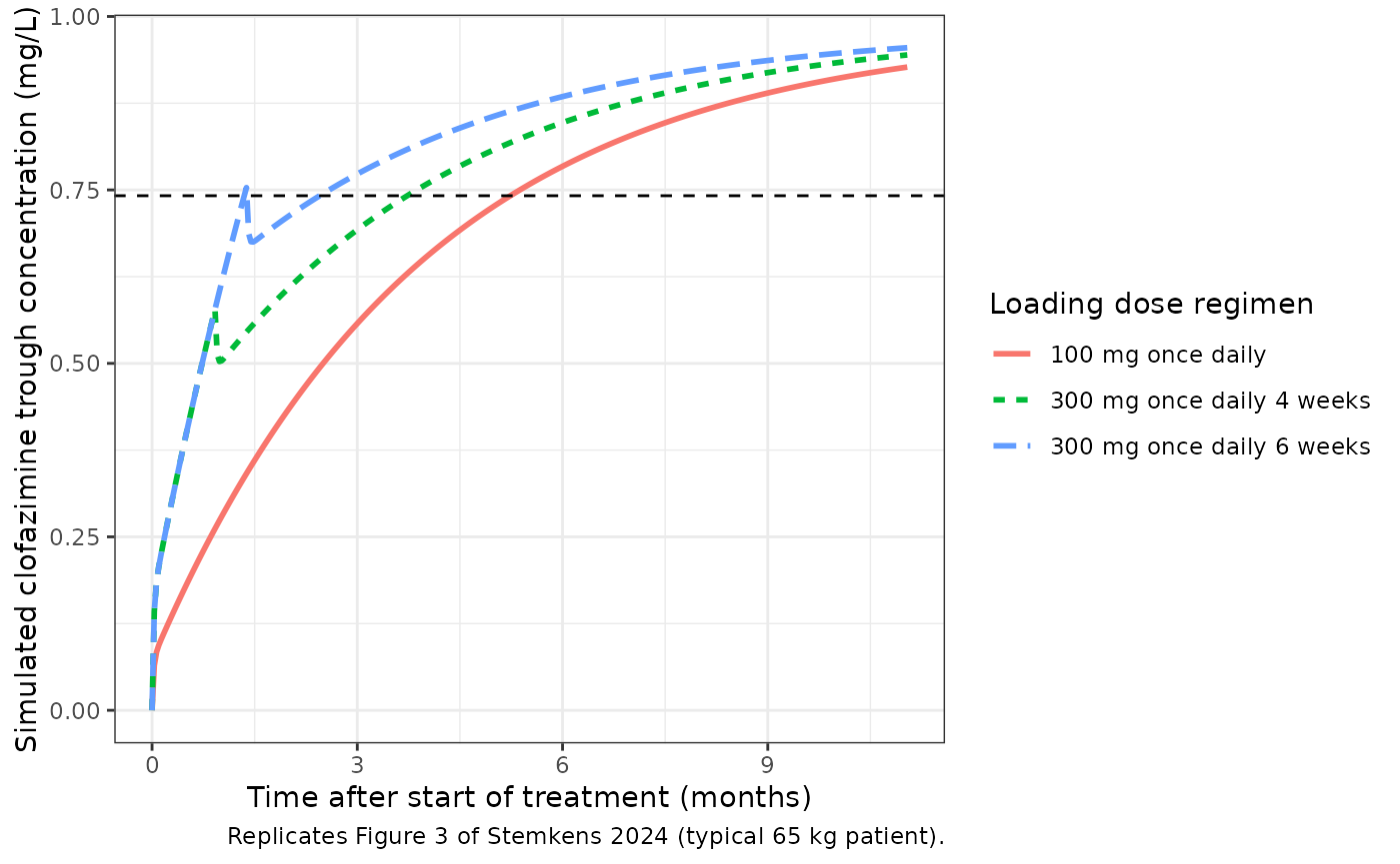
The 100 mg curve ends near 0.93 mg/L at 11 months and the 6-week loading curve peaks at about 0.75 mg/L at the end of loading, as in Figure 3. The dashed target line of Figure 3 sits at about 0.74 mg/L, which is 80% of the trough at the end of the 11-month simulation (0.927 mg/L), not 80% of the true steady-state trough (0.982 mg/L): with an 85-day half-life the 100 mg regimen is still about 6% short of steady state at 11 months. The time-to-target replication below therefore uses the end-of-horizon trough as the “steady-state” reference, which is what reproduces the published numbers.
end_loading <- sim_typical |>
  inner_join(regimens, by = "regimen") |>
  filter(time == loading_weeks * 7 * 24, loading_weeks > 0) |>
  select(regimen, Cc)
end_loading
#>                     regimen        Cc
#> 1 300 mg once daily 4 weeks 0.5778339
#> 2 300 mg once daily 6 weeks 0.7533381
#> 3 300 mg once daily 8 weeks 0.9094765
stopifnot(
  abs(trough_end / 0.93 - 1) < 0.05,
  abs(end_loading$Cc[end_loading$regimen == "300 mg once daily 6 weeks"] / 0.75 - 1) < 0.05
)
ttt_typical <- sim_typical |>
  group_by(regimen) |>
  summarise(months_to_target = min(months[Cc >= target_typical]),
            .groups = "drop") |>
  left_join(
    tibble(regimen = regimens$regimen, table5_median = c(5.3, 3.8, 1.4, 1.4)),
    by = "regimen"
  )
ttt_typical |>
  dplyr::rename("Regimen" = regimen,
                "Typical patient, months to target" = months_to_target,
                "Table 5 median (months)" = table5_median) |>
knitr::kable(digits = 2)| Regimen | Typical patient, months to target | Table 5 median (months) |
|---|---|---|
| 100 mg once daily | 5.26 | 5.3 |
| 300 mg once daily 4 weeks | 3.75 | 3.8 |
| 300 mg once daily 6 weeks | 1.38 | 1.4 |
| 300 mg once daily 8 weeks | 1.38 | 1.4 |
The typical 65 kg patient reaches the target in 5.3, 3.8, 1.4 and 1.4 months on the four regimens, matching the medians of Table 5 to the printed precision. The 4-week and 6-week loading results discriminate sharply between candidate bioavailabilities for the 300 mg dose: the 6-week regimen reaches the target only because the trough at the end of loading just crosses it, which requires the 0.736 relative bioavailability.
Replicate Table 5: virtual population
The paper simulated 1000 patients per regimen with body weight log-normally distributed “based on the combined demographics” of C-LOAD and PERC. The parameters of that distribution are not reported; the cohort below uses a log-normal weight with median 62 kg (the C-LOAD median) and a log-scale SD of 0.2, truncated to 45-120 kg. Each virtual patient keeps the same random effects on every regimen (paired design), drawn in base R so the cohort is identical on every machine, and the individual target is 80% of that patient’s own 100 mg trough at day 336. The cohort has 200 patients per regimen.
set.seed(20241211)
n_pat <- 200
omega_mat <- ui$omega
eta <- matrix(rnorm(n_pat * nrow(omega_mat)), n_pat) %*% chol(omega_mat)
colnames(eta) <- rownames(omega_mat)
wt_pat <- pmin(pmax(exp(rnorm(n_pat, log(62), 0.2)), 45), 120)

ev_pop <- bind_rows(lapply(seq_len(nrow(regimens)), function(i) {
  bind_rows(lapply(seq_len(n_pat), function(k) {
    make_regimen((i - 1) * n_pat + k, regimens$loading_dose[i],
                 regimens$loading_weeks[i], wt = wt_pat[k],
                 regimen = regimens$regimen[i]) |>
      mutate(patient = k)
  }))
}))
params_pop <- data.frame(
  id = (rep(seq_len(nrow(regimens)), each = n_pat) - 1) * n_pat +
    rep(seq_len(n_pat), nrow(regimens)),
  eta[rep(seq_len(n_pat), nrow(regimens)), , drop = FALSE]
)
sim_pop <- solve_long(mod_typical, ev_pop, params = params_pop,
                      keep = c("regimen", "patient")) |>
  mutate(months = time / 24 / 30.4375)
#> Warning: multi-subject simulation without without 'omega'

targets <- sim_pop |>
  filter(regimen == "100 mg once daily", time == horizon_days * 24) |>
  transmute(patient, target = 0.8 * Cc)

ttt_pop <- sim_pop |>
  inner_join(targets, by = "patient") |>
  group_by(regimen, patient) |>
  summarise(months_to_target = min(months[Cc >= target]), .groups = "drop")

table5 <- tibble(
  regimen = regimens$regimen,
  paper = c("5.3 (0.93-8.1)", "3.8 (0.33-7.6)", "1.4 (0.30-7.3)",
            "1.4 (0.30-7.0)"),
  paper_median = c(5.3, 3.8, 1.4, 1.4)
)
ttt_summary <- ttt_pop |>
  group_by(regimen) |>
  summarise(
    median = median(months_to_target),
    p025 = quantile(months_to_target, 0.025),
    p975 = quantile(months_to_target, 0.975),
    .groups = "drop"
  ) |>
  left_join(table5, by = "regimen")
ttt_summary |>
  mutate(simulated = sprintf("%.1f (%.2f-%.1f)", median, p025, p975)) |>
  select(regimen, simulated, paper) |>
  dplyr::rename("Regimen" = regimen,
                "Simulated, months to target, median (2.5th-97.5th)" = simulated,
                "Table 5, median (2.5th-97.5th)" = paper) |>
knitr::kable()| Regimen | Simulated, months to target, median (2.5th-97.5th) | Table 5, median (2.5th-97.5th) |
|---|---|---|
| 100 mg once daily | 5.2 (1.84-8.0) | 5.3 (0.93-8.1) |
| 300 mg once daily 4 weeks | 3.7 (0.30-6.8) | 3.8 (0.33-7.6) |
| 300 mg once daily 6 weeks | 1.3 (0.30-6.2) | 1.4 (0.30-7.3) |
| 300 mg once daily 8 weeks | 1.3 (0.30-5.5) | 1.4 (0.30-7.0) |
# Typical-value medians match Table 5 exactly (above). Across a cohort the
# median moves with which patients land near the threshold, and the 4-week
# regimen sits on a shallow approach to the target, so the band is wider
# there. A wrong clearance, volume or 300 mg bioavailability shifts these
# medians by months, not tenths.
stopifnot(all(abs(ttt_summary$median - ttt_summary$paper_median) < 0.8))
ttt_pop |>
  ggplot(aes(months_to_target, colour = regimen)) +
  stat_ecdf(linewidth = 1) +
  labs(x = "Months to 80% of individual reference trough",
       y = "Cumulative fraction of virtual patients", colour = "Regimen") +
  theme_bw()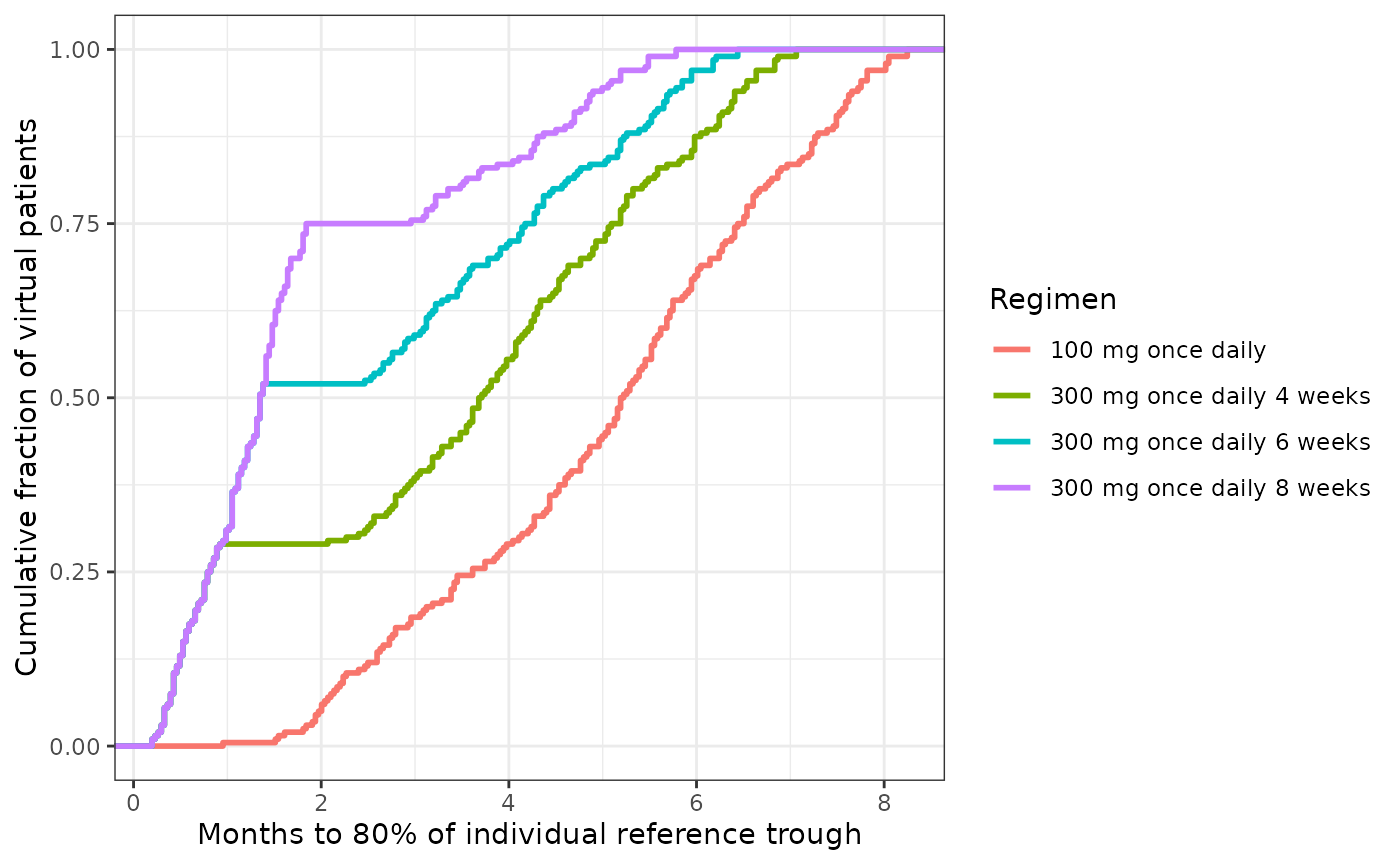
The 200 mg and 400 mg loading regimens of Table 5 are not simulated:
the model’s high-dose bioavailability term is defined only for the 300
mg dose the study used (DOSE_HIGH contrasts 300 mg with 100
mg), and the paper does not report how bioavailability was extrapolated
to 200 mg and 400 mg.
PKNCA validation: model-derived exposure (Table S5)
Table S5 reports geometric means of model-derived AUC0-24h, Cmax,
Tmax and Ctrough at the sampling visits of both studies. The virtual
cohorts below follow the two designs: C-LOAD takes 300 mg once daily for
28 days and then 100 mg once daily; PERC takes 100 mg once daily from
day 0. Each sampled dosing interval is simulated densely, with that
day’s dose carrying its own inter-occasion bioavailability eta, as in
the source data set (OCC 1-3 in C-LOAD, 1-2 in PERC; 0 on
every other dose). Body weight follows the same distribution as above
for both studies.
nca_grid <- c(0, 0.5, 1, 1.5, 2, 3, 4, 5, 6, 7, 8, 10, 12, 16, 20, 24)

make_study <- function(id, study, wt, ndays = 125) {
  dose_day <- 0:(ndays - 1)
  if (study == "C-LOAD") {
    amt <- ifelse(dose_day < 28, 300, 100)
    occ_days <- c(27, 28, 121) # last 300 mg dose, first 100 mg dose, month 4
  } else {
    amt <- rep(100, length(dose_day))
    occ_days <- c(30, 121) # month 1, month 4
  }
  occ <- match(dose_day, occ_days, nomatch = 0L)
  doses <- tibble(
    id = id, time = dose_day * 24, evid = 1L, amt = amt, cmt = "depot",
    DOSE_HIGH = as.integer(amt == 300), OCC = occ
  )
  obs <- tibble(day = rep(occ_days, each = length(nca_grid)),
                tad = rep(nca_grid, length(occ_days))) |>
    mutate(id = id, time = day * 24 + tad, evid = 0L, amt = NA_real_,
           cmt = "central", DOSE_HIGH = NA_integer_, OCC = NA_integer_)
  bind_rows(obs, doses) |>
    arrange(id, time, evid) |>
    tidyr::fill(DOSE_HIGH, OCC, .direction = "up") |>
    tidyr::fill(DOSE_HIGH, OCC, .direction = "down") |>
    mutate(WT = wt, study = study)
}

n_study <- 200
ev_nca <- bind_rows(
  bind_rows(lapply(seq_len(n_study), function(k) make_study(k, "C-LOAD", wt_pat[k]))),
  bind_rows(lapply(seq_len(n_study), function(k) {
    make_study(n_study + k, "PERC", wt_pat[k])
  }))
)
# OCC on an observation row does not enter the model (bioavailability is
# evaluated at the dose); the fill above only keeps the column complete.
params_nca <- data.frame(id = seq_len(2 * n_study),
                         eta[rep(seq_len(n_study), 2), , drop = FALSE])
sim_nca_raw <- solve_long(mod_typical, ev_nca, params = params_nca,
                          keep = "study")
#> Warning: multi-subject simulation without without 'omega'
visit_map <- tibble(
  study = c("C-LOAD", "C-LOAD", "C-LOAD", "PERC", "PERC"),
  day = c(27, 28, 121, 30, 121),
  treatment = c("C-LOAD day 28 (300 mg)", "C-LOAD 1 month (100 mg)",
                "C-LOAD 4 months (100 mg)", "PERC 1 month (100 mg)",
                "PERC 4 months (100 mg)")
)
# Each visit is the 24 h interval starting at that day's dose; the C-LOAD
# day-27 and day-28 intervals share the record at 28 days, hence distinct().
conc_nca <- sim_nca_raw |>
  inner_join(visit_map, by = "study", relationship = "many-to-many") |>
  mutate(tad = time - day * 24) |>
  filter(tad >= 0, tad <= 24, !is.na(Cc)) |>
  distinct(id, treatment, tad, .keep_all = TRUE) |>
  select(id, treatment, time = tad, Cc)
dose_nca <- conc_nca |>
  distinct(id, treatment) |>
  mutate(time = 0, amt = ifelse(grepl("300 mg", treatment), 300, 100))

o_conc <- PKNCA::PKNCAconc(conc_nca, Cc ~ time | treatment + id)
o_dose <- PKNCA::PKNCAdose(dose_nca, amt ~ time | treatment + id)
intervals <- data.frame(start = 0, end = 24, auclast = TRUE, cmax = TRUE,
                        tmax = TRUE, cmin = TRUE)
nca_res <- PKNCA::pk.nca(PKNCA::PKNCAdata(o_conc, o_dose, intervals = intervals))

gm <- function(x) exp(mean(log(x)))
# Tmax is summarised by its median: near steady state some virtual patients
# have a nearly flat profile whose maximum is the pre-dose sample (Tmax = 0),
# and a single zero sends a geometric mean to 0.
sim_gm <- as.data.frame(nca_res$result) |>
  filter(PPTESTCD %in% c("auclast", "cmax", "tmax", "cmin")) |>
  group_by(treatment, PPTESTCD) |>
  summarise(
    PPORRES = if (PPTESTCD[1] == "tmax") median(PPORRES) else gm(PPORRES),
    .groups = "drop"
  )

table_s5 <- tibble(
  treatment = visit_map$treatment,
  auclast = c(16.0, 14.6, 19.8, 7.75, 15.8),
  cmax = c(0.832, 0.734, 0.930, 0.399, 0.767),
  tmax = c(4.28, 3.93, 3.76, 4.99, 5.26),
  cmin = c(0.507, 0.517, 0.716, 0.233, 0.499)
)
cmp <- nlmixr2lib::ncaComparisonTable(
  sim_gm, table_s5, by = "treatment",
  units = c(auclast = "mg*h/L", cmax = "mg/L", tmax = "h", cmin = "mg/L")
)
knitr::kable(cmp, caption = paste(
  "Simulated geometric means (200 virtual patients per study) against the",
  "Table S5 model-derived geometric means (simulated Tmax is the median).",
  "Ctrough of Table S5 is compared with the minimum concentration over the",
  "dosing interval."
))| NCA parameter | treatment | Reference | Simulated | % diff |
|---|---|---|---|---|
| Cmax (mg/L) | C-LOAD day 28 (300 mg) | 0.832 | 0.932 | +12.0% |
| Cmax (mg/L) | C-LOAD 1 month (100 mg) | 0.734 | 0.752 | +2.5% |
| Cmax (mg/L) | C-LOAD 4 months (100 mg) | 0.93 | 0.894 | -3.9% |
| Cmax (mg/L) | PERC 1 month (100 mg) | 0.399 | 0.44 | +10.2% |
| Cmax (mg/L) | PERC 4 months (100 mg) | 0.767 | 0.804 | +4.8% |
| Cmin (mg/L) | C-LOAD day 28 (300 mg) | 0.507 | 0.519 | +2.4% |
| Cmin (mg/L) | C-LOAD 1 month (100 mg) | 0.517 | 0.501 | -3.1% |
| Cmin (mg/L) | C-LOAD 4 months (100 mg) | 0.716 | 0.676 | -5.6% |
| Cmin (mg/L) | PERC 1 month (100 mg) | 0.233 | 0.252 | +8.0% |
| Cmin (mg/L) | PERC 4 months (100 mg) | 0.499 | 0.585 | +17.3% |
| Tmax (h) | C-LOAD day 28 (300 mg) | 4.28 | 5 | +16.8% |
| Tmax (h) | C-LOAD 1 month (100 mg) | 3.93 | 4 | +1.8% |
| Tmax (h) | C-LOAD 4 months (100 mg) | 3.76 | 5 | +33.0%* |
| Tmax (h) | PERC 1 month (100 mg) | 4.99 | 5 | +0.2% |
| Tmax (h) | PERC 4 months (100 mg) | 5.26 | 5 | -4.9% |
| AUClast (mg*h/L) | C-LOAD day 28 (300 mg) | 16 | 18 | +12.5% |
| AUClast (mg*h/L) | C-LOAD 1 month (100 mg) | 14.6 | 15.2 | +3.9% |
| AUClast (mg*h/L) | C-LOAD 4 months (100 mg) | 19.8 | 19.2 | -3.2% |
| AUClast (mg*h/L) | PERC 1 month (100 mg) | 7.75 | 8.57 | +10.5% |
| AUClast (mg*h/L) | PERC 4 months (100 mg) | 15.8 | 17 | +7.5% |
attr(cmp, "footnote")
#> [1] "* differs from reference by more than ±20%."
ratio <- sim_gm |>
  inner_join(tidyr::pivot_longer(table_s5, -treatment, names_to = "PPTESTCD",
                                 values_to = "ref"),
             by = c("treatment", "PPTESTCD")) |>
  filter(PPTESTCD %in% c("auclast", "cmax", "cmin")) |>
  mutate(pct_diff = 100 * (PPORRES / ref - 1))
stopifnot(
  # Centre: a mis-transcribed clearance, dose or bioavailability moves every
  # exposure metric by tens of percent.
  abs(median(ratio$pct_diff)) < 15,
  # Envelope: the Table S5 means come from 8-19 patients per visit with an
  # 85% CV on clearance, so single cells carry wide sampling error.
  quantile(abs(ratio$pct_diff), 0.9) < 35
)
The geometric means of Table S5 come from the empirical Bayes estimates of 8 to 19 patients per visit, with 95% confidence intervals spanning roughly +/-25%; a virtual cohort of 200 with assumed weights is compared against them on the centre of the distribution. The observed geometric means of Table 2 (C-LOAD day 28: Cmax 0.87 mg/L, Ctrough 0.50 mg/L, AUC0-24h 16.1 mg*h/L; highest measured concentration 0.75 and 0.93 mg/L at 1 and 4 months in C-LOAD and 0.39 and 0.78 mg/L in PERC) are close to the Table S5 values and lead to the same conclusion.
Assumptions and deviations
-
Additive residual error. Table 4 prints the
additive error as 0.00174 mg/L, but the same number appears in the Text
S3
$SIGMAblock, where NONMEM reads it as a variance. The proportional term confirms that Table 4 reports$SIGMAon the SD scale (sqrt(0.00639) = 0.080 = the printed 8.00%), so the additive SD is taken from the control stream as sqrt(0.00174) = 0.0417 mg/L. The printed 0.00174 mg/L as an SD would be under 4% of the assay’s 0.05 mg/L lower calibration limit. -
High-dose bioavailability covariate. The control
stream uses a
highdoseflag that is not in its$INPUTlist; the Results describe the contrast as 300 mg versus 100 mg doses. It is encoded per dose record asDOSE_HIGH(1 for a 300 mg dose). The packaged model does not extrapolate to other dose levels, so the 200 mg and 400 mg rows of Table 5 are not replicated. -
Inter-occasion variability on bioavailability
applies only to doses given on PK sampling days (
OCC1-3), as in the source data set;OCC = 0doses have none. Simulations of new regimens setOCC = 0throughout. Whether the paper’s regimen simulations included this term is not stated; it has no effect on the typical-value results above. - “Steady-state” reference for time to target. The target is computed from the 100 mg trough at day 336 (48 weeks, the end of the Figure 3 axis) rather than the true steady state, because that is what reproduces both the Figure 3 target line and the Table 5 medians. The exact simulation horizon is not reported; a month is taken as 30.4375 days.
- Virtual-population body weight. Log-normal with median 62 kg and log-scale SD 0.2, truncated to 45-120 kg; the paper’s distribution parameters are not reported, and PERC demographics are not tabulated.
- Ctrough in the NCA table is compared with the PKNCA minimum concentration over the 24 h interval; Table S5 does not state whether its Ctrough is the pre-dose or end-of-interval value, which differ little near steady state.
- Tmax summary. Table S5 labels its Tmax as a geometric mean; the simulated Tmax is summarised by the median, because virtual patients with a flat steady-state profile have Tmax = 0 and a geometric mean of 0.
-
Covariates screened and not retained (rifampicin
co-administration, age, sex, pulmonary versus extrapulmonary disease,
study) are recorded in the model’s
covariatesDataExcludedmetadata.