Ibrutinib leukocyte, lymph node size and blood pressure dynamics in CLL (Ibrahim 2023)
Source:vignettes/articles/Ibrahim_2023_ibrutinib.Rmd
Ibrahim_2023_ibrutinib.RmdModels and source
This paper contributes four model files to
nlmixr2lib. They were fitted as four separate analyses by
the authors – three in nlmixr and one in msm –
so they are packaged as four files rather than one joint model.
| Model file | Endpoint(s) | Source equations |
|---|---|---|
Ibrahim_2023_ibrutinib_leukocyte_spd |
leukocyte count, SPD | eq. 1 (main text) + eq. S4-S7 (Appendix S2) |
Ibrahim_2023_ibrutinib_sbp |
systolic blood pressure | eq. 2, 3 (main text) |
Ibrahim_2023_ibrutinib_dbp |
diastolic blood pressure | eq. 2, 3 (main text) |
Ibrahim_2023_ibrutinib_competing_risk |
dropout, death | eq. S1-S3 (Appendix S2) |
- Citation: Ibrahim EIK, Karlsson MO, Friberg LE. Assessment of ibrutinib scheduling on leukocyte, lymph node size and blood pressure dynamics in chronic lymphocytic leukemia through pharmacokinetic-pharmacodynamic models. CPT Pharmacometrics Syst Pharmacol. 2023;12(9):1305-1318. doi:10.1002/psp4.13010. Open Access under CC BY-NC. Structural equations from Appendix S2 equations S4-S7 and main-text equation 1; parameter values from the authors’ own nlmixr control stream (Supporting Information S4, run100) cross-checked against Table 1.
- Article: https://doi.org/10.1002/psp4.13010
- Supplement (appendices, tables, figures and the authors’ own
nlmixrcontrol streams): https://doi.org/10.1002/psp4.13010 Supporting Information S1-S4
The parameter values in all four files were taken from the authors’
own nlmixr control streams, published
verbatim as Supporting Information S4. Those streams carry more
significant figures than the rounded values printed in Tables 1 and 2,
and every one of them back-transforms to its table row (see the source trace below).
mLeuk <- rxode2::rxode(modellib("Ibrahim_2023_ibrutinib_leukocyte_spd"))
#> ℹ parameter labels from comments will be replaced by 'label()'
mSbp  <- rxode2::rxode(modellib("Ibrahim_2023_ibrutinib_sbp"))
#> ℹ parameter labels from comments will be replaced by 'label()'
mDbp  <- rxode2::rxode(modellib("Ibrahim_2023_ibrutinib_dbp"))
#> ℹ parameter labels from comments will be replaced by 'label()'
mCr   <- rxode2::rxode(modellib("Ibrahim_2023_ibrutinib_competing_risk"))
Population
The analysis used data from the phase Ib/II study PCYC-1102, which enrolled 132 patients with chronic lymphocytic leukemia (CLL) treated once daily with ibrutinib (420 mg, n = 94; 840 mg, n = 38). The 120 patients who had both leukocyte count and SPD measurements formed the analysis dataset. Baseline characteristics (Supplementary Table S1): mean age 62.4 (SD 9.9) years, mean weight 82.3 (SD 17) kg, 75.8% male, 20.8% treatment-naive and 79.2% relapsed/refractory. Patients were followed for a maximum of 2.4 years (median 1.7 years), with periods of treatment interruption and dose reduction for adverse events. The dataset contained 2374 ibrutinib plasma concentrations, 2434 leukocyte counts, 507 SPD measurements and 2413 paired sBP/dBP measurements; 11 patients died and 22 dropped out (Appendix S1 section 1).
The same information is available programmatically:
str(modellib("Ibrahim_2023_ibrutinib_leukocyte_spd")()$population)
#> List of 11
#>  $ species       : chr "human"
#>  $ n_subjects    : int 120
#>  $ n_studies     : int 1
#>  $ age_range     : chr "mean 62.4 (SD 9.9) years"
#>  $ weight_range  : chr "mean 82.3 (SD 17) kg"
#>  $ sex_female_pct: num 24.2
#>  $ race_ethnicity: NULL
#>  $ disease_state : chr "Chronic lymphocytic leukemia (CLL); 20.8% treatment-naive, 79.2% relapsed/refractory"
#>  $ dose_range    : chr "ibrutinib 420 mg once daily (n = 94) or 840 mg once daily (n = 38) in PCYC-1102; only the 120 patients with bot"| __truncated__
#>  $ regions       : chr "United States (PCYC-1102, phase Ib/II)"
#>  $ notes         : chr "Baseline demographics from Ibrahim 2023 Supplementary Table S1. Follow-up to a maximum of 2.4 years (median 1.7"| __truncated__
Source trace
Structural equations
| Model quantity | Encoded as | Source |
|---|---|---|
Rin,pBTK = kout,pBTK * pBTKbaseline |
kin_pbtk <- kout_pbtk * pbtk_base |
eq. 1 |
EFF = IMAX * AUC / (IAUC50 + AUC) |
effauc <- imax_pbtk * AUC_IBRU / (iauc50_pbtk + AUC_IBRU) |
eq. 1 |
d(pBTK)/dt = Rin*(1-EFF) - kout*pBTK |
d/dt(pbtk) |
eq. 1 |
pBTKeff = pBTKbaseline - pBTK |
pbtk_eff <- pbtk_base - pbtk |
Appendix S2 |
resist = exp(-lambda_dec * t) |
resist <- exp(-lambda_dec * t) |
Appendix S2 |
CLLsubpop,3,baseline = frc2 * CLLtiss,baseline |
cll_subpop3_base <- frc2 * clltiss0 |
main text (kdist definition) |
kdist = (kh + kd,bld) * CLLbld,baseline / CLLsubpop,3,baseline |
kdist <- (kh + kd_bld) * (cllbld0 / cll_subpop3_base) |
main text (kdist definition) |
d(CLLsubpop,1)/dt |
d/dt(cll_subpop1) |
eq. S4 |
d(CLLsubpop,2)/dt |
d/dt(cll_subpop2) |
eq. S5 |
d(CLLsubpop,3)/dt |
d/dt(cll_subpop3) |
eq. S6 |
d(CLLbld)/dt |
d/dt(cll_bld) |
eq. S7 |
SCcells-SPD = SPDbaseline / CLLtiss,baseline |
sc_cells_spd <- spdbase / clltiss0 |
Results, “PK-SPD-leukocyte model” |
kdtch = kp |
kdtch <- kp |
Table 1 footnote c |
| leukocyte = (CLLbld + NRMbld) / VBld | leukocyte <- (cll_bld + nrmbld) / vbld |
Figure 1 caption |
| SPD = CLLsubpop,1+2+3 + NRMLN | tumorSpd <- ... + nrmln |
Figure 1 caption |
Rin,iBP = kout,iBP * iBPbaseline |
kin_sbp <- sbpbase * kout_sbp |
eq. 2 |
EFF = Emax*AUC / (AUC50 + AUC) |
effauc <- emax_sbp * AUC_IBRU / (auc50_sbp + AUC_IBRU) |
eq. 2 |
d(transit)/dt = Rin*(1+EFF) - ktr*transit |
d/dt(transit1) |
eq. 2 |
d(iBP)/dt = ktr*transit - kout*iBP |
d/dt(sbp), d/dt(dbp)
|
eq. 3 |
ktr,iBP = (n+1)/MTT, n = 1 |
ktr_sbp <- ntransit_sbp / mtt_sbp |
main text, “PK-blood pressure model” |
MTTsBP = e^(LN(79.9) - 5.04*LN(Age/63)) |
mtt_sbp <- exp(lmtt_sbp + eta + e_age_mtt_sbp*log(AGE/63)) |
Table 2 footnote c |
dBPbaseline = e^(LN(69.7) - 0.204*LN(Age/63)) |
dbpbase <- exp(lrbase_dbp + eta + e_age_base_dbp*log(AGE/63)) |
Table 2 footnote b |
d(S1)/dt = -lambda12*S1 - lambda13*S1 |
d/dt(s_alive) |
eq. S1 |
d(S2)/dt = lambda12*S1 |
d/dt(s_dropout) |
eq. S2 |
d(S3)/dt = lambda13*S1 |
d/dt(s_death) |
eq. S3 |
lambda12 = 0.00908 * e^(-0.89*LN(Leukocyte/12)) |
lambda12 <- exp(llambda12)*exp(e_wbc_lambda12*log(WBC/12)) |
Table 2 footnote e |
lambda13 = 0.00275 * e^(0.563*LN(SPD/14) + 1.42*del(17p)) |
lambda13 <- ... |
Table 2 footnote f |
Parameters: control stream vs. published table
Every log-scale THETA in the model files is the value printed in the
authors’ nlmixr control stream (Supporting Information S4).
This chunk back-transforms each one and compares it against the
corresponding Table 1 / Table 2 row.
trace <- tibble::tribble(
  ~model,        ~parameter,        ~theta,        ~published, ~table,
  "leuk/SPD", "kout,pBTK",         0.2986911,      1.35,      "Table 1",
  "leuk/SPD", "CLLbld,0",          4.1644135,      64.1,      "Table 1",
  "leuk/SPD", "CLLtiss,baseline",  7.6449086,      2090,      "Table 1",
  "leuk/SPD", "SPDunm,baseline",   3.8860955,      48.9,      "Table 1",
  "leuk/SPD", "SPDm,baseline",     2.9725082,      19.5,      "Table 1",
  "leuk/SPD", "NRMbld,TN",         3.4941826,      32.9,      "Table 1",
  "leuk/SPD", "NRMbld,RR",         2.8503700,      17.3,      "Table 1",
  "leuk/SPD", "NRMLN",             0.7843116,      2.19,      "Table 1",
  "leuk/SPD", "kp",               -5.4811627,      0.00416,   "Table 1",
  "leuk/SPD", "kh",               -0.7571987,      0.469,     "Table 1",
  "leuk/SPD", "kd,bld",           -4.8761701,      0.00763,   "Table 1",
  "leuk/SPD", "kd,tiss",          -1.7320378,      0.177,     "Table 1",
  "leuk/SPD", "IAUC50,pBTK",       3.5299932,      34.1,      "Table 1",
  "leuk/SPD", "slp2",              2.4260423,      11.3,      "Table 1",
  "leuk/SPD", "slp3",             -2.3192759,      0.0983,    "Table 1",
  "leuk/SPD", "lambda_dec",       -7.0012733,      0.000911,  "Table 1",
  "sBP",      "sBPbaseline",       4.83995310,     126,       "Table 2",
  "sBP",      "MTTsBP",            4.38126172,     79.9,      "Table 2",
  "sBP",      "Emax,sBP",         -2.17877709,     0.113,     "Table 2",
  "sBP",      "AUC50,sBP",         4.51798998,     91.7,      "Table 2",
  "dBP",      "dBPbaseline",       4.24388453,     69.7,      "Table 2",
  "dBP",      "MTTdBP",            5.08188777,     161,       "Table 2",
  "dBP",      "Emax,dBP",         -2.66779698,     0.0694,    "Table 2",
  "dBP",      "AUC50,dBP",         4.14476079,     63.1,      "Table 2"
) |>
  mutate(
    back_transformed = exp(theta),
    pct_diff = 100 * (back_transformed - published) / published
  )

trace |>
  mutate(across(c(back_transformed, published), ~ signif(.x, 4)),
         pct_diff = round(pct_diff, 2)) |>
  dplyr::rename("Model" = model, "Parameter" = parameter,
                "log-scale THETA (S4)" = theta,
                "exp(THETA)" = back_transformed,
                "Published" = published, "Source" = table,
                "% difference" = pct_diff) |>
knitr::kable()| Model | Parameter | log-scale THETA (S4) | Published | Source | exp(THETA) | % difference |
|---|---|---|---|---|---|---|
| leuk/SPD | kout,pBTK | 0.2986911 | 1.35e+00 | Table 1 | 1.348e+00 | -0.14 |
| leuk/SPD | CLLbld,0 | 4.1644135 | 6.41e+01 | Table 1 | 6.435e+01 | 0.40 |
| leuk/SPD | CLLtiss,baseline | 7.6449086 | 2.09e+03 | Table 1 | 2.090e+03 | 0.00 |
| leuk/SPD | SPDunm,baseline | 3.8860955 | 4.89e+01 | Table 1 | 4.872e+01 | -0.37 |
| leuk/SPD | SPDm,baseline | 2.9725082 | 1.95e+01 | Table 1 | 1.954e+01 | 0.21 |
| leuk/SPD | NRMbld,TN | 3.4941826 | 3.29e+01 | Table 1 | 3.292e+01 | 0.07 |
| leuk/SPD | NRMbld,RR | 2.8503700 | 1.73e+01 | Table 1 | 1.729e+01 | -0.03 |
| leuk/SPD | NRMLN | 0.7843116 | 2.19e+00 | Table 1 | 2.191e+00 | 0.04 |
| leuk/SPD | kp | -5.4811627 | 4.16e-03 | Table 1 | 4.164e-03 | 0.11 |
| leuk/SPD | kh | -0.7571987 | 4.69e-01 | Table 1 | 4.690e-01 | 0.00 |
| leuk/SPD | kd,bld | -4.8761701 | 7.63e-03 | Table 1 | 7.626e-03 | -0.05 |
| leuk/SPD | kd,tiss | -1.7320378 | 1.77e-01 | Table 1 | 1.769e-01 | -0.04 |
| leuk/SPD | IAUC50,pBTK | 3.5299932 | 3.41e+01 | Table 1 | 3.412e+01 | 0.07 |
| leuk/SPD | slp2 | 2.4260423 | 1.13e+01 | Table 1 | 1.131e+01 | 0.12 |
| leuk/SPD | slp3 | -2.3192759 | 9.83e-02 | Table 1 | 9.834e-02 | 0.05 |
| leuk/SPD | lambda_dec | -7.0012733 | 9.11e-04 | Table 1 | 9.107e-04 | -0.03 |
| sBP | sBPbaseline | 4.8399531 | 1.26e+02 | Table 2 | 1.265e+02 | 0.37 |
| sBP | MTTsBP | 4.3812617 | 7.99e+01 | Table 2 | 7.994e+01 | 0.05 |
| sBP | Emax,sBP | -2.1787771 | 1.13e-01 | Table 2 | 1.132e-01 | 0.16 |
| sBP | AUC50,sBP | 4.5179900 | 9.17e+01 | Table 2 | 9.165e+01 | -0.05 |
| dBP | dBPbaseline | 4.2438845 | 6.97e+01 | Table 2 | 6.968e+01 | -0.03 |
| dBP | MTTdBP | 5.0818878 | 1.61e+02 | Table 2 | 1.611e+02 | 0.05 |
| dBP | Emax,dBP | -2.6677970 | 6.94e-02 | Table 2 | 6.940e-02 | 0.01 |
| dBP | AUC50,dBP | 4.1447608 | 6.31e+01 | Table 2 | 6.310e+01 | 0.00 |
All parameters agree to within rounding except the two whose random
effects are Box-Cox transformed (CLLbld,0 and
SPDbaseline), where the published table reports the typical
value implied by the Box-Cox random-effect distribution rather than the
raw structural THETA. The logit-scale fractions and the derived
half-lives reproduce the paper’s prose exactly:
frc <- function(x) exp(x) / (1 + exp(x))
tibble::tibble(
  Quantity = c("frc1", "frc2", "kd,tiss half-life (day)", "kd,bld half-life (day)",
               "resistance half-life (day)", "slp2 / slp3",
               "detachment enhancement, subpop 1 (fold)",
               "detachment enhancement, subpop 2 (fold)",
               "SPD unmutated / mutated (fold)", "NRMbld TN / RR (fold)",
               "MTT dBP / sBP (fold)"),
  Reproduced = c(frc(-0.1152389), frc(-1.3357462),
                 log(2) / exp(-1.7320378), log(2) / exp(-4.8761701),
                 log(2) / exp(-7.0012733), exp(2.4260423) / exp(-2.3192759),
                 1 + exp(2.4260423), 1 + exp(-2.3192759),
                 48.9 / 19.5, 32.9 / 17.3, 161 / 79.9),
  Paper = c(0.471, 0.208, 3.92, 90.8, 761, 115, 12.3, 1.1, 2.5, 1.9, 2.01)
) |>
  mutate(Reproduced = signif(Reproduced, 4)) |>
knitr::kable()| Quantity | Reproduced | Paper |
|---|---|---|
| frc1 | 0.4712 | 0.471 |
| frc2 | 0.2082 | 0.208 |
| kd,tiss half-life (day) | 3.9180 | 3.920 |
| kd,bld half-life (day) | 90.8900 | 90.800 |
| resistance half-life (day) | 761.1000 | 761.000 |
| slp2 / slp3 | 115.0000 | 115.000 |
| detachment enhancement, subpop 1 (fold) | 12.3100 | 12.300 |
| detachment enhancement, subpop 2 (fold) | 1.0980 | 1.100 |
| SPD unmutated / mutated (fold) | 2.5080 | 2.500 |
| NRMbld TN / RR (fold) | 1.9020 | 1.900 |
| MTT dBP / sBP (fold) | 2.0150 | 2.010 |
Units
Ibrutinib never appears as a concentration in any of these models – it enters only through the daily-AUC covariate – so a units table replaces the usual concentration bookkeeping.
| Symbol | Units | Note |
|---|---|---|
t (leuk/SPD, sBP, dBP) |
day | |
t (competing risk) |
month | lambda12/lambda13 are per month (Table 2) |
AUC_IBRU |
h*ng/mL | daily AUC(0-24) |
pbtk |
relative (1 = 100% phosphorylated) |
pBTKbaseline fixed to 100% |
cll_subpop1, cll_subpop2,
cll_subpop3
|
cm^2 | carried on the SPD scale |
cll_bld |
10^9 cells | carried on the cell-count scale |
leukocyte |
10^9 cells/L |
(cll_bld + nrmbld) / vbld, vbld = 5 L |
tumorSpd |
cm^2 | |
sbp, dbp
|
mmHg | |
kp, kh, kd_bld,
kd_tiss, kdist, kdtch,
kout_pbtk, lambda_dec
|
1/day | |
sc_cells_spd |
cm^2 / 10^9 cells | bridges the two measurement scales |
sc_spd_cells |
10^9 cells / cm^2 | reciprocal |
s_alive, s_dropout, s_death,
sur
|
probability |
The two scale factors are what make the mixed-unit ODE system
dimensionally consistent: in eq. S6 the homing influx
kh * cll_bld * sc_cells_spd converts
(1/day) * 10^9 cells * (cm^2 / 10^9 cells) = cm^2/day,
matching d(cll_subpop3)/dt; in eq. S7 the redistribution
influx kdist * cll_subpop3 * sc_spd_cells converts
(1/day) * cm^2 * (10^9 cells / cm^2) = 10^9 cells/day,
matching d(cll_bld)/dt.
The exposure input
All three PK-PD models are driven by the daily AUC(0-24) of
ibrutinib, which Ibrahim 2023 obtained by integrating individual post
hoc profiles of the two-compartment ibrutinib population PK model of
Marostica et al. (Cancer Chemother Pharmacol. 2015;75(1):111-121). That
upstream PK model is not part of
nlmixr2lib and the paper does not tabulate the resulting
AUC values, so the AUC per dose level has to be recovered from the paper
itself.
The paper does report median steady-state Btk occupancy at the end of
cycle 3 for each simulated schedule. Occupancy is defined as
(1 - pBtk) * 100, and at steady state the pBtk turnover
model collapses to pBtk = 1 - EFF, so
occupancy / 100 = EFF = AUC / (IAUC50 + AUC) => AUC = IAUC50 * occ / (1 - occ)which inverts exactly for a typical patient (IAUC50 =
34.1 h*ng/mL).
iauc50 <- exp(3.5299932)          # IAUC50,pBTK, S4 run100 tic50
schedules <- tibble::tibble(
  dose_mg   = c(420, 280, 140),
  occupancy = c(0.927, 0.894, 0.808)   # Results: 92.7%, 89.4%, 80.8%
) |>
  mutate(
    auc = iauc50 * occupancy / (1 - occupancy),
    auc_per_mg = auc / dose_mg
  )

schedules |>
  mutate(across(c(auc, auc_per_mg), ~ signif(.x, 4))) |>
  dplyr::rename("Dose (mg/day)" = dose_mg, "Reported Btk occupancy" = occupancy,
                "Implied AUC(0-24) (h*ng/mL)" = auc,
                "AUC per mg" = auc_per_mg) |>
knitr::kable()| Dose (mg/day) | Reported Btk occupancy | Implied AUC(0-24) (h*ng/mL) | AUC per mg |
|---|---|---|---|
| 420 | 0.927 | 433.3 | 1.032 |
| 280 | 0.894 | 287.8 | 1.028 |
| 140 | 0.808 | 143.6 | 1.026 |
The three independently-derived AUC values are proportional to dose
to within 0.6% (AUC per mg = 1.032, 1.028, 1.026), which is
a meaningful consistency check: the three occupancy figures were
reported separately, the inversion uses only IAUC50, and
dose-proportional ibrutinib PK is exactly what the upstream Marostica
model would produce. This supports using these AUC values as the
exposure input below. They are nonetheless derived, not
published values – see Assumptions and
deviations.
aucFor <- setNames(schedules$auc, schedules$dose_mg)
# The three schedules compared by the paper; one cycle = 28 days.
aucSchedule <- function(time, schedule) {
  cycle <- floor(time / 28) + 1
  if (schedule == "420 mg/day (approved)") {
    rep(aucFor[["420"]], length(time))
  } else if (schedule == "de-escalation 1") {
    ifelse(cycle <= 1, aucFor[["420"]], aucFor[["280"]])
  } else {
    ifelse(cycle <= 1, aucFor[["420"]],
           ifelse(cycle <= 2, aucFor[["280"]], aucFor[["140"]]))
  }
}
schedLevels <- c("420 mg/day (approved)", "de-escalation 1", "de-escalation 2")
PK-SPD-leukocyte model
Drug-free behaviour and the pseudo-steady-state construction
With AUC_IBRU = 0 there is no drug effect at all, so
pbtk must sit exactly at its baseline of 1 and the
peripheral-blood pool must be at steady state – that is precisely what
the paper’s kdist definition enforces. Algebraically, at t
= 0 and zero exposure, eq. S7 reduces to
kdist * CLLsubpop,3(0) * SC_SPD-cells
  = (kh + kd,bld) * (CLLbld,0 / (frc2*CLLtiss,0)) * (SPDbaseline*frc2) * (CLLtiss,0/SPDbaseline)
  = (kh + kd,bld) * CLLbld,0
which cancels exactly against the efflux
(kh + kd,bld) * CLLbld(0). The tissue pool, by contrast, is
not at steady state – untreated CLL grows – and eq. S6 reduces
to SPDbaseline * (kp - kd,bld * CLLbld,0 / CLLtiss,0), a
positive growth rate. Both are confirmed numerically:
typLeuk <- rxode2::zeroRe(mLeuk, which = c("omega", "sigma"))

obsGrid <- function(times) {
  tibble::tibble(time = times, evid = 0L, cmt = "cll_bld", dvid = 1L)
}

evFree <- obsGrid(seq(0, 730, by = 7)) |>
  mutate(AUC_IBRU = 0, TUM_IGHV_MUT = 0, LINE_1L = 0)
simFree <- rxode2::rxSolve(typLeuk$simulationModel, evFree,
                           useLinCmt = FALSE, returnType = "data.frame")
#> ℹ omega/sigma items treated as zero: 'etalrbase_cllbld', 'etalrbase_clltiss', 'etalnrmbld', 'etalkd_bld', 'etalkh', 'etalkd_tiss', 'etalkp', 'etalogit_frc1', 'etalogit_frc2', 'etaliauc50_pbtk', 'etalkout_pbtk', 'etallambda_dec', 'etalrbase_spd', 'etalnrmln'

# 1. pBtk is invariant without drug
stopifnot(isTRUE(all.equal(range(simFree$pbtk), c(1, 1), tolerance = 1e-8)))

# 2. the blood pool flux balance holds at t = 0
row0 <- simFree[simFree$time == 0, ]
influx  <- row0$kdist * row0$cll_subpop3 * row0$sc_spd_cells
efflux  <- (row0$kh + row0$kd_bld) * row0$cll_bld
stopifnot(isTRUE(all.equal(influx, efflux, tolerance = 1e-8)))

# 3. the predicted tissue growth rate matches the algebra above
predictedGrowth <- row0$spdbase * (row0$kp - row0$kd_bld * row0$cllbld0 / row0$clltiss0)

tibble::tibble(
  Check = c("pBtk range without drug", "blood-pool influx at t=0",
            "blood-pool efflux at t=0", "tissue growth rate at t=0 (cm^2/day)"),
  Value = c(paste(signif(range(simFree$pbtk), 8), collapse = " to "),
            signif(influx, 6), signif(efflux, 6), signif(predictedGrowth, 6))
) |>
knitr::kable()| Check | Value |
|---|---|
| pBtk range without drug | 1 to 1 |
| blood-pool influx at t=0 | 30.6718 |
| blood-pool efflux at t=0 | 30.6718 |
| tissue growth rate at t=0 (cm^2/day) | 0.191454 |
Left untreated for two years the model therefore predicts progressive disease, which is the correct biological behaviour:
tibble::tibble(
  Output = c("leukocyte (10^9/L)", "total SPD (cm^2)"),
  `Day 0` = signif(c(simFree$leukocyte[1], simFree$tumorSpd[1]), 4),
  `Day 730` = signif(c(dplyr::last(simFree$leukocyte), dplyr::last(simFree$tumorSpd)), 4)
) |>
knitr::kable()| Output | Day 0 | Day 730 |
|---|---|---|
| leukocyte (10^9/L) | 16.33 | 485.5 |
| total SPD (cm^2) | 50.91 | 423.1 |
Btk occupancy reproduces the published values
Running the typical-value model on each schedule and reading off Btk occupancy on the last day of cycle 3 (day 84) reproduces the paper’s reported medians – as it must, since the AUC inputs were inverted from exactly those numbers. This is therefore a round-trip check on the Imax encoding rather than an independent validation.
occSim <- lapply(schedLevels, function(s) {
  ev <- obsGrid(seq(0, 84, by = 1)) |>
    mutate(AUC_IBRU = aucSchedule(time, s), TUM_IGHV_MUT = 0, LINE_1L = 0)
  out <- rxode2::rxSolve(typLeuk$simulationModel, ev, useLinCmt = FALSE,
                         returnType = "data.frame")
  tibble::tibble(schedule = s, occupancy_day84 = dplyr::last(out$btkOccupancy))
}) |> bind_rows()
#> ℹ omega/sigma items treated as zero: 'etalrbase_cllbld', 'etalrbase_clltiss', 'etalnrmbld', 'etalkd_bld', 'etalkh', 'etalkd_tiss', 'etalkp', 'etalogit_frc1', 'etalogit_frc2', 'etaliauc50_pbtk', 'etalkout_pbtk', 'etallambda_dec', 'etalrbase_spd', 'etalnrmln'
#> ℹ omega/sigma items treated as zero: 'etalrbase_cllbld', 'etalrbase_clltiss', 'etalnrmbld', 'etalkd_bld', 'etalkh', 'etalkd_tiss', 'etalkp', 'etalogit_frc1', 'etalogit_frc2', 'etaliauc50_pbtk', 'etalkout_pbtk', 'etallambda_dec', 'etalrbase_spd', 'etalnrmln'
#> ℹ omega/sigma items treated as zero: 'etalrbase_cllbld', 'etalrbase_clltiss', 'etalnrmbld', 'etalkd_bld', 'etalkh', 'etalkd_tiss', 'etalkp', 'etalogit_frc1', 'etalogit_frc2', 'etaliauc50_pbtk', 'etalkout_pbtk', 'etallambda_dec', 'etalrbase_spd', 'etalnrmln'

occSim |>
  mutate(published = c(92.7, 89.4, 80.8),
         occupancy_day84 = round(occupancy_day84, 1)) |>
  dplyr::rename("Schedule" = schedule, "Simulated Btk occupancy (%)" = occupancy_day84,
                "Published (%)" = published) |>
knitr::kable()| Schedule | Simulated Btk occupancy (%) | Published (%) |
|---|---|---|
| 420 mg/day (approved) | 92.7 | 92.7 |
| de-escalation 1 | 89.4 | 89.4 |
| de-escalation 2 | 80.8 | 80.8 |
Treatment-related lymphocytosis
The model’s signature behaviour is the transient rise in blood leukocyte count caused by ibrutinib blocking CLL cells from homing back to lymphoid tissue while simultaneously accelerating their detachment from the stroma – the cells are redistributed into blood, where they “die by neglect” with a 90.8-day half-life.
evTreat <- obsGrid(seq(0, 730, by = 2)) |>
  mutate(AUC_IBRU = aucFor[["420"]], TUM_IGHV_MUT = 0, LINE_1L = 0)
simTreat <- rxode2::rxSolve(typLeuk$simulationModel, evTreat,
                            useLinCmt = FALSE, returnType = "data.frame")
#> ℹ omega/sigma items treated as zero: 'etalrbase_cllbld', 'etalrbase_clltiss', 'etalnrmbld', 'etalkd_bld', 'etalkh', 'etalkd_tiss', 'etalkp', 'etalogit_frc1', 'etalogit_frc2', 'etaliauc50_pbtk', 'etalkout_pbtk', 'etallambda_dec', 'etalrbase_spd', 'etalnrmln'

simTreat |>
  select(time, `Leukocyte (10^9/L)` = leukocyte, `Total SPD (cm^2)` = tumorSpd) |>
  pivot_longer(-time, names_to = "output", values_to = "value") |>
  ggplot(aes(time, value)) +
  geom_line(linewidth = 0.8) +
  facet_wrap(~output, scales = "free_y") +
  labs(x = "Time (days)", y = NULL) +
  theme_bw()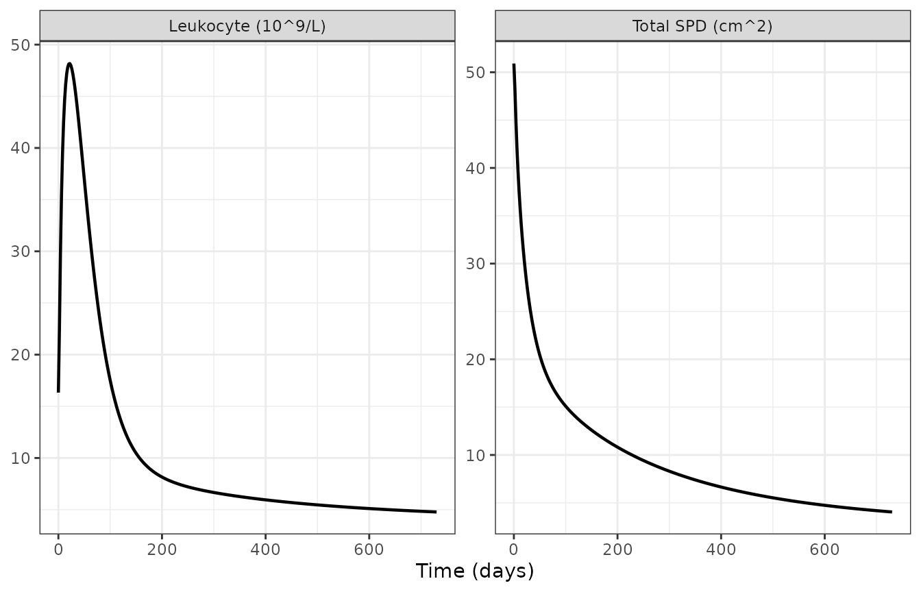
Typical-value leukocyte count and total SPD on the approved 420 mg/day schedule. The early leukocyte peak is the treatment-related lymphocytosis described in Ibrahim 2023.
tibble::tibble(
  Quantity = c("Baseline leukocyte (10^9/L)", "Peak leukocyte (10^9/L)",
               "Day of peak", "Leukocyte at 2 years (10^9/L)",
               "SPD change at 2 years (%)"),
  Value = c(signif(simTreat$leukocyte[1], 4),
            signif(max(simTreat$leukocyte), 4),
            simTreat$time[which.max(simTreat$leukocyte)],
            signif(dplyr::last(simTreat$leukocyte), 4),
            round(100 * (dplyr::last(simTreat$tumorSpd) / simTreat$tumorSpd[1] - 1), 1))
) |>
knitr::kable()| Quantity | Value |
|---|---|
| Baseline leukocyte (10^9/L) | 16.330 |
| Peak leukocyte (10^9/L) | 48.170 |
| Day of peak | 22.000 |
| Leukocyte at 2 years (10^9/L) | 4.779 |
| SPD change at 2 years (%) | -92.100 |
Replication of Figure 4: total CLL burden by dosing schedule
Figure 4 of Ibrahim 2023 summarises the relative change of the
individual predictions of total CLL count from
baseline, with the median and the 10th and 90th percentiles, for the
three schedules. totalCll is exposed by the model file (the
three lymphoid-tissue subpopulations converted to the cell scale plus
the peripheral-blood pool).
nSub <- 200L   # per arm

cohort <- tibble::tibble(
  id = seq_len(nSub),
  TUM_IGHV_MUT = rbinom(nSub, 1, 0.35),
  LINE_1L      = rbinom(nSub, 1, 0.208)   # 20.8% treatment-naive (Table S1)
)

simSchedule <- function(s, times = seq(0, 730, by = 10)) {
  ev <- tidyr::expand_grid(id = cohort$id, time = times) |>
    arrange(id, time) |>
    left_join(cohort, by = "id") |>
    mutate(evid = 0L, cmt = "cll_bld", dvid = 1L,
           AUC_IBRU = aucSchedule(time, s))
  # Re-seeding before every arm makes the three schedules share one set of
  # eta realisations, so they are compared on the *same* virtual patients --
  # as in Ibrahim 2023, which simulated replicates of the original dataset and
  # re-ran each schedule on them. Without pairing, the between-schedule
  # differences are smaller than the Monte-Carlo noise at this cohort size.
  set.seed(20230909)
  # `omega` is passed explicitly. rxode2 otherwise re-uses the random-effect
  # settings of the last model solved off the same compiled ODE system, and
  # the typical-value (zeroRe) runs above would silently zero the IIV here.
  rxode2::rxSolve(mLeuk$simulationModel, ev, omega = mLeuk$omega,
                  useLinCmt = FALSE, returnType = "data.frame") |>
    mutate(schedule = s)
}

simPop <- lapply(schedLevels, simSchedule) |> bind_rows()
stopifnot(!anyNA(simPop$totalCll))
# Guard: confirm between-subject variability was actually sampled. If this
# fails the "population" simulation collapsed onto a single typical subject.
stopifnot(n_distinct(round(simPop$iauc50_pbtk, 8)) > 1)

relChange <- simPop |>
  group_by(schedule, id) |>
  arrange(time, .by_group = TRUE) |>
  mutate(rel = 100 * (totalCll / first(totalCll) - 1)) |>
  ungroup() |>
  group_by(schedule, time) |>
  summarise(p10 = quantile(rel, 0.10), p50 = median(rel),
            p90 = quantile(rel, 0.90), .groups = "drop") |>
  mutate(schedule = factor(schedule, levels = schedLevels))

ggplot(relChange, aes(time, p50, colour = schedule)) +
  geom_line(linewidth = 0.9) +
  geom_line(aes(y = p10), linetype = "dashed") +
  geom_line(aes(y = p90), linetype = "dashed") +
  scale_colour_manual(values = c("#d62728", "#1f77b4", "#7f7f7f")) +
  labs(x = "Time (days)", y = "Relative change in total CLL count (%)",
       colour = "Schedule") +
  theme_bw() + theme(legend.position = "bottom")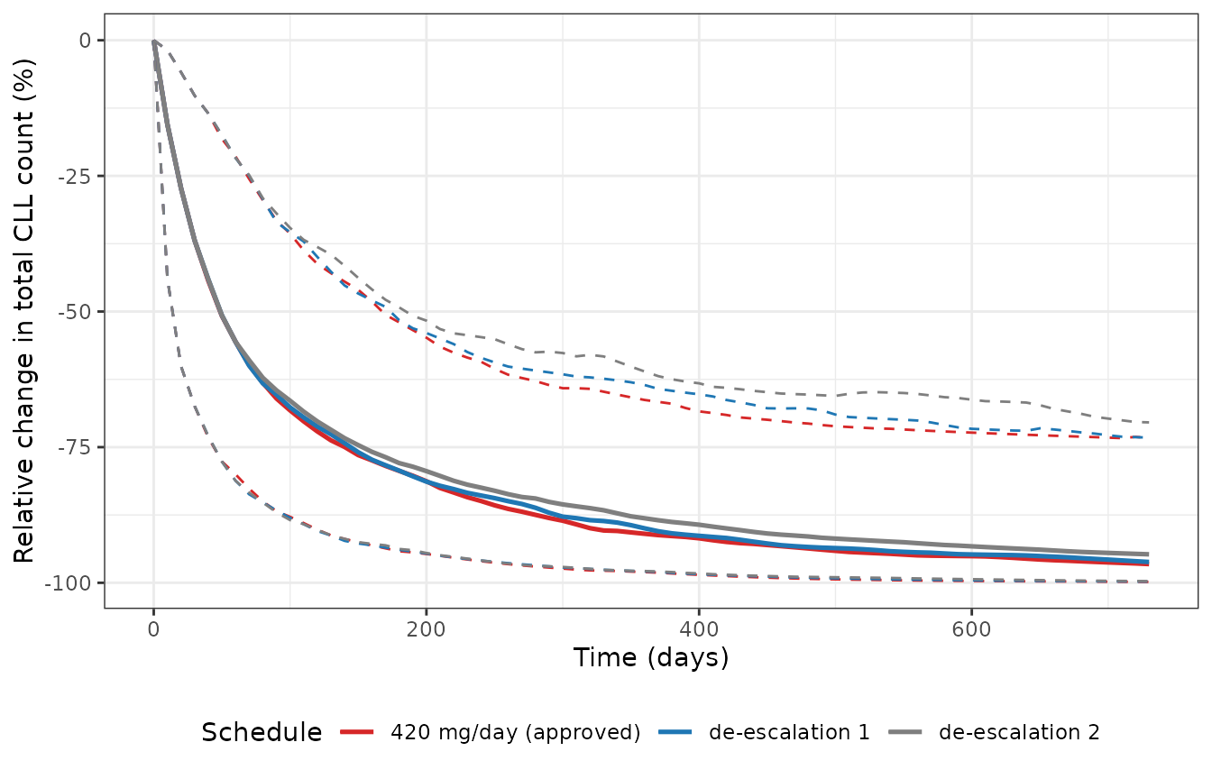
Replicates Figure 4 of Ibrahim 2023: relative change of total CLL count from baseline. Solid lines are medians, dashed lines the 10th and 90th percentiles. One cycle is 28 days.
The ordering the paper reports is reproduced: the approved schedule gives the largest reduction in total tumour burden and de-escalation schedule 2 the smallest, with the differences concentrated in the upper percentile.
relChange |>
  filter(time == 730) |>
  mutate(across(c(p10, p50, p90), ~ round(.x, 1))) |>
  dplyr::rename("Schedule" = schedule, "Day" = time,
                "10th pct (%)" = p10, "Median (%)" = p50, "90th pct (%)" = p90) |>
knitr::kable()| Schedule | Day | 10th pct (%) | Median (%) | 90th pct (%) |
|---|---|---|---|---|
| 420 mg/day (approved) | 730 | -99.8 | -96.5 | -73.3 |
| de-escalation 1 | 730 | -99.8 | -96.2 | -73.2 |
| de-escalation 2 | 730 | -99.7 | -94.7 | -70.4 |
PK-blood pressure models
Algebraic check on the plateau
At steady state both blood-pressure models plateau at
iBPbaseline * (1 + Emax*AUC/(AUC50 + AUC)). This is a
closed-form target the simulation must hit.
typSbp <- rxode2::zeroRe(mSbp, which = c("omega", "sigma"))
typDbp <- rxode2::zeroRe(mDbp, which = c("omega", "sigma"))

bpGrid <- function(times, age) {
  tibble::tibble(time = times, evid = 0L,
                 AUC_IBRU = aucFor[["420"]], AGE = age)
}
sSbp <- rxode2::rxSolve(typSbp, bpGrid(seq(0, 1460, by = 5), 63),
                        useLinCmt = FALSE, returnType = "data.frame")
#> ℹ omega/sigma items treated as zero: 'etalrbase_sbp', 'etalmtt_sbp', 'etalemax_sbp'
sDbp <- rxode2::rxSolve(typDbp, bpGrid(seq(0, 1460, by = 5), 63),
                        useLinCmt = FALSE, returnType = "data.frame")
#> ℹ omega/sigma items treated as zero: 'etalrbase_dbp', 'etalemax_dbp'

expected <- function(base, emax, auc50) {
  base * (1 + emax * aucFor[["420"]] / (auc50 + aucFor[["420"]]))
}
tibble::tibble(
  Model = c("sBP", "dBP"),
  `Baseline (mmHg)` = signif(c(sSbp$sbp[1], sDbp$dbp[1]), 5),
  `Simulated plateau (mmHg)` = signif(c(dplyr::last(sSbp$sbp), dplyr::last(sDbp$dbp)), 5),
  `Closed-form plateau (mmHg)` = signif(c(
    expected(exp(4.83995310), exp(-2.17877709), exp(4.51798998)),
    expected(exp(4.24388453), exp(-2.66779698), exp(4.14476079))), 5)
) |>
knitr::kable()| Model | Baseline (mmHg) | Simulated plateau (mmHg) | Closed-form plateau (mmHg) |
|---|---|---|---|
| sBP | 126.460 | 138.280 | 138.280 |
| dBP | 69.678 | 73.899 | 73.899 |
Replication of Figure 5: proportion of patients with hypertension
Figure 5 of Ibrahim 2023 gives the proportion of patients with sBP >= 140 mmHg and dBP >= 90 mmHg over time for the three schedules. The paper also reports the values at baseline and at 2 years, which are the quantitative targets here.
bpCohort <- tibble::tibble(
  id  = seq_len(nSub),
  AGE = pmax(30, rnorm(nSub, mean = 62.4, sd = 9.9))   # Table S1
)

simBp <- function(mod, s, times = seq(0, 730, by = 10)) {
  ev <- tidyr::expand_grid(id = bpCohort$id, time = times) |>
    arrange(id, time) |>
    left_join(bpCohort, by = "id") |>
    mutate(evid = 0L, AUC_IBRU = aucSchedule(time, s))
  # Re-seed for arm pairing and pass `omega` explicitly, for the same reasons
  # as in the Figure 4 chunk.
  set.seed(20230909)
  rxode2::rxSolve(mod, ev, omega = mod$omega, useLinCmt = FALSE,
                  returnType = "data.frame") |>
    mutate(schedule = s)
}

sbpPop <- lapply(schedLevels, function(s) simBp(mSbp, s)) |> bind_rows()
dbpPop <- lapply(schedLevels, function(s) simBp(mDbp, s)) |> bind_rows()
stopifnot(!anyNA(sbpPop$sbp), !anyNA(dbpPop$dbp))
# Guard: confirm between-subject variability was actually sampled.
stopifnot(n_distinct(round(sbpPop$sbpbase, 8)) > 1,
          n_distinct(round(dbpPop$dbpbase, 8)) > 1)

props <- bind_rows(
  sbpPop |> group_by(schedule, time) |>
    summarise(prop = 100 * mean(sbp >= 140), .groups = "drop") |>
    mutate(endpoint = "sBP >= 140 mmHg"),
  dbpPop |> group_by(schedule, time) |>
    summarise(prop = 100 * mean(dbp >= 90), .groups = "drop") |>
    mutate(endpoint = "dBP >= 90 mmHg")
) |>
  mutate(schedule = factor(schedule, levels = schedLevels))
ggplot(props, aes(time, prop, colour = schedule)) +
  geom_line(linewidth = 0.9) +
  facet_wrap(~endpoint, scales = "free_y") +
  scale_colour_manual(values = c("#d62728", "#1f77b4", "#7f7f7f")) +
  labs(x = "Time (days)", y = "Patients (%)", colour = "Schedule") +
  theme_bw() + theme(legend.position = "bottom")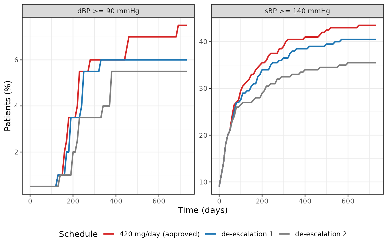
Replicates Figure 5 of Ibrahim 2023: predicted proportion of patients with (a) sBP >= 140 mmHg and (b) dBP >= 90 mmHg. One cycle is 28 days.
published <- tibble::tribble(
  ~endpoint,         ~schedule,               ~time, ~published,
  "sBP >= 140 mmHg", "420 mg/day (approved)",  0,    10.2,
  "sBP >= 140 mmHg", "420 mg/day (approved)",  730,  44.7,
  "sBP >= 140 mmHg", "de-escalation 1",        730,  41.1,
  "sBP >= 140 mmHg", "de-escalation 2",        730,  34.7,
  "dBP >= 90 mmHg",  "420 mg/day (approved)",  0,    0.25,
  "dBP >= 90 mmHg",  "420 mg/day (approved)",  730,  7.83,
  "dBP >= 90 mmHg",  "de-escalation 1",        730,  6.92,
  "dBP >= 90 mmHg",  "de-escalation 2",        730,  4.75
)

props |>
  mutate(schedule = as.character(schedule)) |>
  inner_join(published, by = c("endpoint", "schedule", "time")) |>
  mutate(simulated = round(prop, 1), .keep = "unused") |>
  arrange(endpoint, time, schedule) |>
  select(endpoint, schedule, time, simulated, published) |>
  dplyr::rename("Endpoint" = endpoint, "Schedule" = schedule, "Day" = time,
                "Simulated (%)" = simulated, "Published (%)" = published) |>
knitr::kable()| Endpoint | Schedule | Day | Simulated (%) | Published (%) |
|---|---|---|---|---|
| dBP >= 90 mmHg | 420 mg/day (approved) | 0 | 0.5 | 0.25 |
| dBP >= 90 mmHg | 420 mg/day (approved) | 730 | 7.5 | 7.83 |
| dBP >= 90 mmHg | de-escalation 1 | 730 | 6.0 | 6.92 |
| dBP >= 90 mmHg | de-escalation 2 | 730 | 5.5 | 4.75 |
| sBP >= 140 mmHg | 420 mg/day (approved) | 0 | 9.0 | 10.20 |
| sBP >= 140 mmHg | 420 mg/day (approved) | 730 | 43.5 | 44.70 |
| sBP >= 140 mmHg | de-escalation 1 | 730 | 40.5 | 41.10 |
| sBP >= 140 mmHg | de-escalation 2 | 730 | 35.5 | 34.70 |
The baseline proportions are an especially clean check because they
depend only on the baseline distributions, with no exposure term:
analytically,
P(sBP >= 140) = P(Z >= log(140/126.46)/0.0827) = 10.9%
against a published 10.2%, and P(dBP >= 90) is a few
tenths of a percent against a published 0.25%. The 2-year values are
simulated from a 200-patient cohort per arm, so they carry Monte-Carlo
noise of a few percentage points; the ordering across the three
schedules (approved > de-escalation 1 > de-escalation 2) is the
paper’s central safety finding and is reproduced.
Competing risk model
Mass balance and reproduction of the published hazard ratios
The three states must always sum to 1, and the covariate coefficients must reproduce the hazard ratios quoted in the Results.
crGrid <- function(times, wbc, spd_cm2, del17p) {
  tibble::tibble(time = times, evid = 0L, WBC = wbc,
                 TUMSZ = spd_cm2 * 100,   # cm^2 -> mm^2 (canonical TUMSZ unit)
                 TUM_17P_DEL = del17p)
}
typCr <- rxode2::zeroRe(mCr, which = c("omega", "sigma"))
#> Warning: No omega parameters in the model
crRef <- rxode2::rxSolve(typCr, crGrid(seq(0, 30, by = 0.5), 12, 14, 0),
                         useLinCmt = FALSE, returnType = "data.frame")

massBalance <- max(abs(crRef$s_alive + crRef$s_dropout + crRef$s_death - 1))
stopifnot(massBalance < 1e-8)

hrGrid <- function(wbc, spd_cm2, del17p) {
  rxode2::rxSolve(typCr, crGrid(c(0, 1), wbc, spd_cm2, del17p),
                  useLinCmt = FALSE, returnType = "data.frame")[1, ]
}
ref  <- hrGrid(12, 14, 0)
hrWbc  <- hrGrid(2, 14, 0)$lambda12  / ref$lambda12    # 10-unit DECREASE in leukocyte
hrSpd  <- hrGrid(12, 24, 0)$lambda13 / ref$lambda13    # 10-unit INCREASE in SPD
hrDel  <- hrGrid(12, 14, 1)$lambda13 / ref$lambda13    # del(17p) present

tibble::tibble(
  Check = c("max |S1 + S2 + S3 - 1|",
            "HR, 10-unit decrease in leukocyte count (on dropout)",
            "HR, 10-unit increase in SPD (on death)",
            "HR, deletion(17p) (on death)"),
  Simulated = c(format(massBalance, digits = 3),
                signif(hrWbc, 4), signif(hrSpd, 4), signif(hrDel, 4)),
  Published = c("(exact)", "4.92", "1.35", "4.16")
) |>
knitr::kable()| Check | Simulated | Published |
|---|---|---|
| max |S1 + S2 + S3 - 1| | 1.11e-15 | (exact) |
| HR, 10-unit decrease in leukocyte count (on dropout) | 4.927 | 4.92 |
| HR, 10-unit increase in SPD (on death) | 1.355 | 1.35 |
| HR, deletion(17p) (on death) | 4.137 | 4.16 |
Replication of Figure 3: dropout and overall-survival curves
Figure 3 of Ibrahim 2023 shows Kaplan-Meier visual predictive checks for dropout probability and overall survival over the study period. Holding the two time-varying predictors at their reference values reproduces the shape and magnitude of both curves.
crCurves <- bind_rows(
  crRef |> mutate(group = "no del(17p)"),
  rxode2::rxSolve(typCr, crGrid(seq(0, 30, by = 0.5), 12, 14, 1),
                  useLinCmt = FALSE, returnType = "data.frame") |>
    mutate(group = "del(17p)")
)

crCurves |>
  select(time, group, `Dropout probability` = probDropout, `Overall survival` = sur) |>
  pivot_longer(c(-time, -group), names_to = "curve", values_to = "value") |>
  ggplot(aes(time, value, colour = group)) +
  geom_line(linewidth = 0.9) +
  facet_wrap(~curve, scales = "free_y") +
  scale_colour_manual(values = c("#d62728", "#1f77b4")) +
  labs(x = "Time (months)", y = "Probability", colour = NULL) +
  theme_bw() + theme(legend.position = "bottom")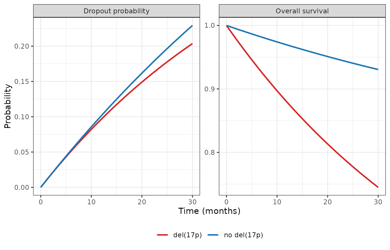
Replicates Figure 3 of Ibrahim 2023: model-predicted dropout probability (left) and overall survival (right) over 30 months, at the reference leukocyte count (12 x10^9/L) and SPD (14 cm^2), with and without deletion(17p).
crCurves |>
  filter(time %in% c(12, 24)) |>
  transmute(group, Month = time,
            `Dropout (%)` = round(100 * probDropout, 1),
            `Death (%)` = round(100 * probDeath, 1),
            `Overall survival (%)` = round(100 * sur, 1)) |>
  dplyr::rename("Group" = group) |>
knitr::kable()| Group | Month | Dropout (%) | Death (%) | Overall survival (%) |
|---|---|---|---|---|
| no del(17p) | 12 | 10.2 | 3.1 | 96.9 |
| no del(17p) | 24 | 19.0 | 5.7 | 94.3 |
| del(17p) | 12 | 9.7 | 12.1 | 87.9 |
| del(17p) | 24 | 17.2 | 21.6 | 78.4 |
At the reference covariate values the model predicts roughly 5-6% mortality and 19% dropout by 24 months, which is the right magnitude for a cohort in which 11 of 120 patients died and 22 dropped out over a median 1.7 years of follow-up (Appendix S1 section 1).
Why there is no PKNCA section
The usual PKNCA validation does not apply to this paper. None of the
four models contains a drug compartment, a dosing event, or a plasma
concentration: ibrutinib enters only as the daily-AUC covariate
AUC_IBRU, and every model output is a biomarker (leukocyte
count, lymph-node area, blood pressure) or a state-occupancy
probability. There is no concentration-time profile to integrate.
Following the endogenous / mechanistic validation strategy instead, this
vignette uses the drug-free invariance and flux-balance checks,
closed-form plateau and hazard-ratio checks, a dimensional analysis of
the mixed-unit ODE system, and replication of the paper’s Figures 3, 4
and 5.
Assumptions and deviations
-
The daily AUC(0-24) values are derived, not
published. Ibrahim 2023 drove all three PK-PD models with
per-subject AUC(0-24) integrated from the Marostica 2015 two-compartment
ibrutinib popPK model, which is not in
nlmixr2liband whose AUC output the paper does not tabulate. The values used in this vignette (433, 288 and 144 h*ng/mL for 420, 280 and 140 mg/day) were inverted from the paper’s own reported median Btk occupancies through the exact steady-state relation of the pBtk model (see The exposure input). The inversion is exact for a typical patient but the reported occupancies are population medians, so a subject with an atypicalIAUC50would map to a different AUC. The three values are dose-proportional to within 0.6%, which supports the derivation. The model files themselves contain no AUC values –AUC_IBRUis a covariate column that the user supplies. -
The three schedules are compared on a paired cohort of 200
patients per arm. Each arm is re-seeded before solving so that
all three schedules use the same eta realisations, mirroring Ibrahim
2023’s design of generating replicates of the original dataset and
re-running each schedule on them. Without pairing, the between-schedule
differences – which are only a few percentage points – are smaller than
the Monte-Carlo noise at this cohort size and the published ordering
does not reliably emerge. Population
rxSolve()calls also passomegaexplicitly, because rxode2 otherwise re-uses the random-effect settings of the last model solved from the same compiled ODE system, which would silently zero the IIV after the typical-value runs. Both chunks assert that between-subject variability was actually sampled. - Population simulations use assumed covariate distributions. Age was drawn as N(62.4, 9.9) truncated at 30 years and treatment-naive status as Bernoulli(0.208), both from Supplementary Table S1. The IGHV-mutated fraction is not reported in the available Table S1 excerpt, so 35% was assumed for the Figure 4 cohort; it affects only the baseline-SPD mixture and not any conclusion drawn here.
-
TUMSZis registered in mm^2, the paper reports SPD in cm^2. The competing-risk model’s SPD predictor is stored under the canonicalTUMSZcolumn, whose registered unit is mm^2, so the reference value is 1400 mm^2 (= the paper’s 14 cm^2). Because the effect is a power form the conversion is numerically invariant, but the sister modelIbrahim_2023_ibrutinib_leukocyte_spdemitstumorSpdin cm^2 and must be multiplied by 100 before being fed here – as done in the chunks above. -
LINE_1Lis the inverse of the paper’sTRTARMcolumn. The authors’ control stream codesTRTARM = 0for treatment-naive; the canonicalLINE_1Lcodes 1 for treatment-naive. Ingestion must applyLINE_1L = 1 - TRTARM. -
Residual error is encoded as log-normal rather than
additive-on-log. Both tables state that the additive RUV model
was implemented on log-transformed data, and the authors’ code emits
log(output + 1e-6)with an additive residual. That is exactly nlmixr2’slnorm()residual, so the model files keep the outputs in their natural units (cm^2, 10^9 cells/L, mmHg) and attachlnorm(). The1e-6numerical guard is not needed and was dropped. -
The competing-risk model carries a placeholder
residual. The source analysis maximised a multistate event
likelihood in
msmand has no observation-error model. A tiny additive residual (addSd = 0.001) is attached tosurso the nlmixr2 likelihood machinery accepts the model for forward simulation. This value is not from the paper. -
The del(17p) coefficient is placed on the death
hazard. Table 2 labels the row “Coefficient of deletion (17p)
on lambda12”, but footnote f writes the term inside the
lambda13equation and the Results narrative states that del(17p) patients had a higher probability of death. The footnote equation and the narrative agree with each other against the row label, so the coefficient is encoded onlambda13. - The competing-risk model runs on a month axis. Its transition rate constants are per month (Table 2), whereas the three PK-PD models are per day. Coupling them requires a time-unit conversion, done explicitly in the chunks above.
-
Antihypertensive co-medication and sex are documented but
not encoded. Both were screened as candidate covariates in the
blood-pressure models and neither was retained; the paper reports no
coefficient for either, so they are recorded under
covariatesDataExcludedrather thancovariateData. Deletion(11q) and deletion(13q) were likewise screened and not retained. -
Ibrahim_2023_ibrutinib_leukocyte_spduses$simulationModel. The model has two endpoints (leukocyteandtumorSpd); observation rows therefore carry both a namedcmtand advid, and allrxSolve()calls passuseLinCmt = FALSE.