Clonidine in ICU adults (Cloesmeijer 2020)
Source:vignettes/articles/Cloesmeijer_2020_clonidine.Rmd
Cloesmeijer_2020_clonidine.RmdModel and source
- Citation: Cloesmeijer ME, van den Oever HLA, Mathot RAA, Zeeman M, Kruisdijk-Gerritsen A, Bles CMA, Nassikovker P, de Meijer AR, van Steveninck FL, Arbouw MEL. Optimising the dose of clonidine to achieve sedation in intensive care unit patients with population pharmacokinetics. Br J Clin Pharmacol. 2020;86(8):1620-1631. doi:10.1111/bcp.14273.
- Description: Two-compartment population PK model for intravenous clonidine in critically ill, intubated and sedated adult intensive care unit patients receiving continuous IV infusion (600-1800 ug/day, with or without a 4-h loading infusion). Central volume is allometrically scaled to body weight with a fixed exponent of 1 (reference 70 kg); clearance increases linearly with time after the start of the clonidine infusion (0.213 percent per hour). IIV on CL and V1 only; combined additive and proportional residual error.
- Article: https://doi.org/10.1111/bcp.14273 (open access, PMC7373711)
Cloesmeijer et al. developed a two-compartment population PK model for intravenous clonidine given as an add-on sedative to intubated adults in the intensive care unit. The final model (Table 2 model 9, Table 3) has two covariate relationships:
- central volume V1 is scaled to body weight with a fixed exponent of
1,
V1 = 124 L * (WT/70); - clearance rises linearly with time after the start of the clonidine
infusion,
CL = 17.0 L/h * (1 + 0.00213 * t), so the typical CL of 17.0 L/h at the start of treatment has risen to 20.5 L/h after 4 days.
IIV is on CL and V1 only, and the residual error is combined additive and proportional.
Population
Twenty-four intubated, sedated adults admitted to the ICU of Deventer Hospital (The Netherlands; NCT02466373) with an expected stay of at least 3 days received clonidine on top of standard sedation with morphine plus midazolam or propofol. Eight patients each received a continuous infusion of 600, 1200 or 1800 ug/day (25, 50 or 75 ug/h); in each group four of the eight also received a loading dose of 50% of the daily dose over 4 h. Table 1 reports 16 men and 8 women, median age 67 (25-83) years, weight 84 (53-113) kg, BMI 27 (20-44) kg/m^2, serum creatinine 74 (32-441) umol/L and albumin 20 (12-32) g/L; three patients received continuous veno-venous haemofiltration. The median treatment duration was 96 (25-171) h. 275 plasma concentrations (5-16 per patient) were analysed; the 11 below the 0.1 ug/L LLOQ were discarded in the final model.
The same information is available programmatically via
rxode2::rxode(readModelDb("Cloesmeijer_2020_clonidine"))$population.
Source trace
Every ini() line in
inst/modeldb/specificDrugs/Cloesmeijer_2020_clonidine.R
carries an in-file source-location comment. The table below collects
them.
| Equation / parameter | Value | Source location |
|---|---|---|
Two-compartment IV model, d/dt(central),
d/dt(peripheral1)
|
n/a | Results 3.1.1; Table 3 |
Log-normal IIV, theta_i = theta_pop * exp(eta_i)
|
n/a | Methods Eq 1 |
| Combined additive + proportional residual error | n/a | Methods Eqs 2-3; Results 3.1.1 |
V1 allometric scaling (WT/70)^1, exponent fixed |
e_wt_vc = 1 (fixed) |
Methods 2.3.2 Eq 4 and text; Results 3.1.3 |
Linear effect of time after start of infusion on CL,
CL * (1 + slope * t)
|
n/a | Methods Eq 6 and text; Table 2 model 9 |
lcl (CL at the start of the infusion) |
log(17.0 L/h) | Table 3 |
lvc (V1 for a 70 kg patient) |
log(124 L) | Table 3 |
lq (Q) |
log(83.7 L/h) | Table 3 |
lvp (V2) |
log(178 L) | Table 3 |
cl_time_slope (fractional increase in CL per hour) |
0.00213 1/h | Table 3 ‘Increase CL per hour 0.213’, stated as percent per hour in the Discussion |
etalcl (IIV CL) |
33.3% CV -> 0.105189 | Table 3 |
etalvc (IIV V1) |
66.8% CV -> 0.369689 | Table 3 |
propSd |
0.141 (fraction) | Table 3 |
addSd |
0.0532 ug/L | Table 3 |
Virtual cohort
The observed data are not public. Section 2.5 of the paper describes the Monte Carlo cohort behind Figure 4: body weight “followed a normal distribution from 53 to 113 kg with a mean of 84 kg”. The standard deviation is not stated; the cohort below uses 15 kg (a quarter of the range) and redraws any value outside 53-113 kg.
Two simulated designs are used:
-
Figure 4 regimens (200 subjects per regimen, 4 days
of infusion):
- 50 ug/h; (B) 50 ug/h plus a 150 ug bolus given over 30 min at the start;
- 100 ug/h for 6 h, then 50 ug/h.
- The study design (100 subjects per arm, six arms): 25, 50 or 75 ug/h for 96 h (the median treatment duration), with or without a preceding 4-h loading infusion of half the daily dose, followed by 48 h of washout.
# set.seed() fixes R's draws of body weight. It does not fix rxode2's
# simulation RNG across solver thread counts, so every assertion below is
# written to hold for any cohort the model can produce.
set.seed(20200514)

draw_wt <- function(n) {
  wt <- rnorm(n, mean = 84, sd = 15)
  while (any(out <- wt < 53 | wt > 113)) {
    wt[out] <- rnorm(sum(out), mean = 84, sd = 15)
  }
  wt
}

# One row per infusion segment for each regimen. `amt` is the total amount
# given in the segment and `rate` the ug/h infusion rate.
fig4_doses <- list(
  "A: 50 ug/h" = tibble(time = 0, amt = 50 * 96, rate = 50),
  "B: 50 ug/h + 150 ug over 30 min" = tibble(
    time = c(0, 0), amt = c(150, 50 * 96), rate = c(300, 50)
  ),
  "C: 100 ug/h for 6 h, then 50 ug/h" = tibble(
    time = c(0, 6), amt = c(100 * 6, 50 * 90), rate = c(100, 50)
  )
)

make_arm <- function(doses, label, n, id_offset, obs_times) {
  ids <- id_offset + seq_len(n)
  subj <- tibble(id = ids, WT = draw_wt(n))
  dose_rows <- tidyr::crossing(subj, doses) |>
    mutate(evid = 1L, cmt = "central")
  obs_rows <- tidyr::crossing(subj, time = obs_times) |>
    mutate(amt = NA_real_, rate = NA_real_, evid = 0L, cmt = "central")
  bind_rows(dose_rows, obs_rows) |>
    mutate(regimen = label) |>
    arrange(id, time, desc(evid))
}

fig4_times <- sort(unique(c(seq(0, 24, by = 0.25), seq(24, 96, by = 1))))
fig4_events <- bind_rows(lapply(seq_along(fig4_doses), function(i) {
  make_arm(fig4_doses[[i]], names(fig4_doses)[i],
    n = 200, id_offset = (i - 1) * 200, obs_times = fig4_times
  )
}))

# Study design: 96 h of maintenance infusion, optionally preceded by a 4-h
# loading infusion of 50% of the daily dose, then 48 h of washout.
study_doses <- list()
for (rate in c(25, 50, 75)) {
  study_doses[[sprintf("%d ug/h", rate)]] <-
    tibble(time = 0, amt = rate * 96, rate = rate)
  study_doses[[sprintf("%d ug/h + loading", rate)]] <- tibble(
    time = c(0, 4),
    amt = c(0.5 * rate * 24, rate * 92),
    rate = c(0.5 * rate * 24 / 4, rate)
  )
}
study_times <- sort(unique(c(seq(0, 12, by = 0.25), seq(12, 144, by = 1))))
study_events <- bind_rows(lapply(seq_along(study_doses), function(i) {
  make_arm(study_doses[[i]], names(study_doses)[i],
    n = 100, id_offset = 10000 + (i - 1) * 100, obs_times = study_times
  )
})) |>
  mutate(
    maint_rate = as.numeric(sub(" ug/h.*$", "", regimen)),
    loading = grepl("loading", regimen)
  )

stopifnot(
  length(unique(fig4_events$id)) == 600,
  length(unique(study_events$id)) == 600,
  !anyNA(fig4_events$WT),
  all(fig4_events$WT >= 53 & fig4_events$WT <= 113)
)
Simulation
mod <- readModelDb("Cloesmeijer_2020_clonidine")

rxode2::rxSetSeed(20200514)
sim_fig4 <- rxode2::rxSolve(mod, events = fig4_events, keep = c("regimen", "WT")) |>
  as.data.frame()
#> ℹ parameter labels from comments will be replaced by 'label()'
sim_study <- rxode2::rxSolve(
  mod,
  events = study_events,
  keep = c("regimen", "WT", "maint_rate", "loading")
) |>
  as.data.frame()

stopifnot(!anyNA(sim_fig4$Cc), !anyNA(sim_study$Cc))
Replicate Figure 4 – dosing simulations
fig4_summary <- sim_fig4 |>
  group_by(regimen, time) |>
  summarise(
    p05 = quantile(sim, 0.05),
    p50 = median(sim),
    p95 = quantile(sim, 0.95),
    .groups = "drop"
  )

ggplot(fig4_summary, aes(time, p50)) +
  geom_ribbon(aes(ymin = p05, ymax = p95), fill = "grey80") +
  geom_line() +
  geom_hline(yintercept = c(1.5, 4), linetype = "dashed", colour = "grey40") +
  facet_wrap(~regimen, ncol = 1) +
  scale_x_continuous(breaks = seq(0, 96, 12)) +
  labs(x = "Time after start of infusion (h)", y = "Clonidine (ug/L)")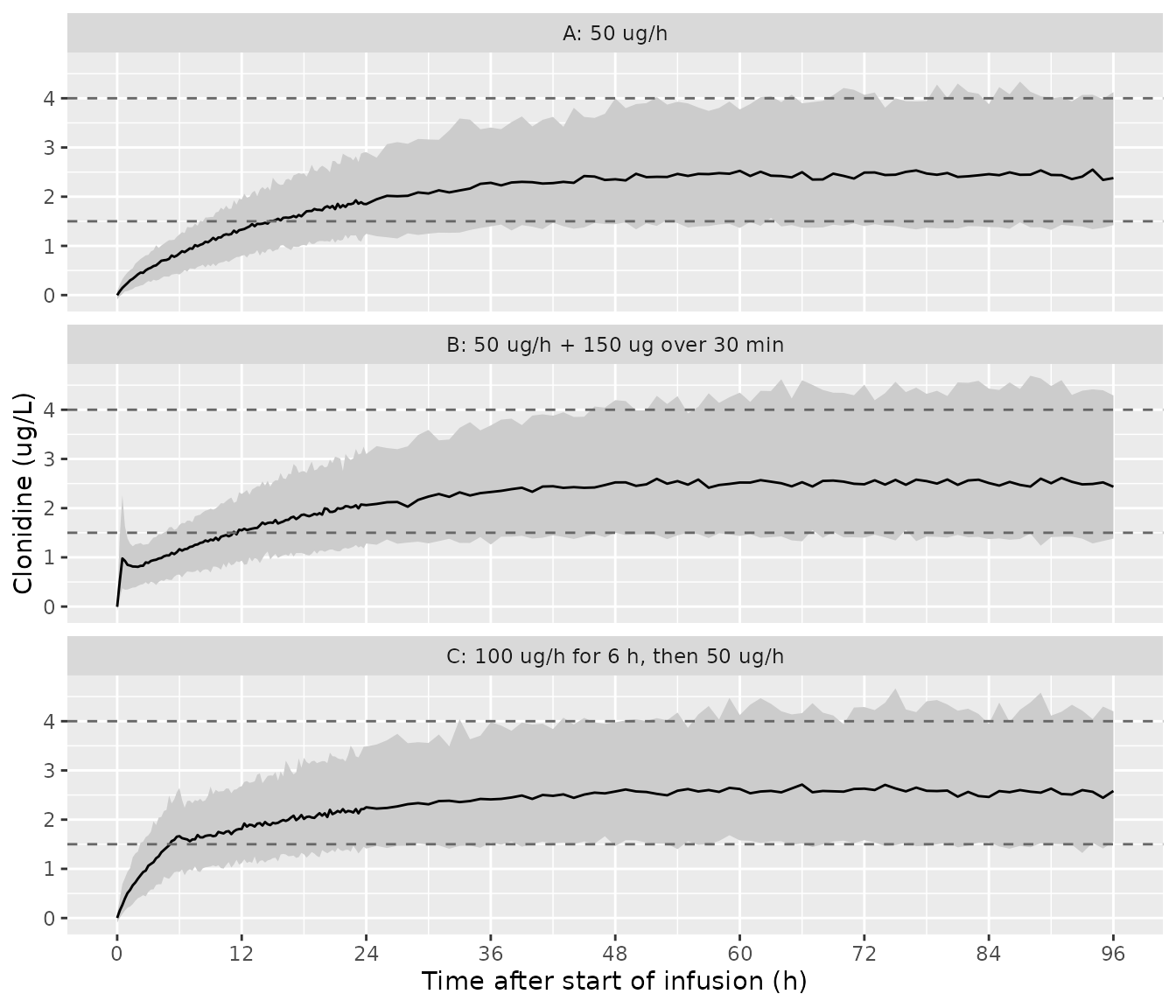
Replicates Figure 4 of Cloesmeijer 2020: median and 5th-95th percentile clonidine concentrations (with residual error) for three regimens over 4 days. Dashed lines mark the 1.5-4.0 ug/L target range.
The paper quotes three numbers from these simulations: the time for 50% of the population to reach 1.5 ug/L (14.5, 11 and 5 h for regimens A, B and C) and, for regimen A, that 95% of patients are above 1.5 ug/L at steady state.
time_to_target <- fig4_summary |>
  group_by(regimen) |>
  summarise(simulated_h = min(time[p50 >= 1.5]), .groups = "drop") |>
  mutate(published_h = c(14.5, 11, 5))

# Individual predictions (no residual error) for the steady-state claim.
# Clearance keeps rising, so the "steady state" is a slowly falling plateau;
# report the fraction above target on days 2, 3 and 4.
above_target <- sim_fig4 |>
  filter(regimen == names(fig4_doses)[1], time %in% c(48, 72, 96)) |>
  group_by(time) |>
  summarise(pct_above_1.5 = 100 * mean(ipredSim > 1.5), .groups = "drop")

time_to_target |>
  dplyr::rename(
    "Regimen" = regimen,
    "Simulated median time to 1.5 ug/L (h)" = simulated_h,
    "Published (h)" = published_h
  ) |>
knitr::kable(caption = "Time for the median concentration to reach 1.5 ug/L (Results 3.2).")| Regimen | Simulated median time to 1.5 ug/L (h) | Published (h) |
|---|---|---|
| A: 50 ug/h | 14.75 | 14.5 |
| B: 50 ug/h + 150 ug over 30 min | 11.25 | 11.0 |
| C: 100 ug/h for 6 h, then 50 ug/h | 5.25 | 5.0 |
above_target |>
  dplyr::rename(
    "Time after start (h)" = time,
    "Percent of subjects above 1.5 ug/L" = pct_above_1.5
  ) |>
  knitr::kable(
    digits = 1,
    caption = "Regimen A, percent of simulated subjects above 1.5 ug/L; published 95% at steady state.",
    row.names = FALSE
)| Time after start (h) | Percent of subjects above 1.5 ug/L |
|---|---|
| 48 | 95.0 |
| 72 | 95.5 |
| 96 | 94.5 |
stopifnot(
  nrow(time_to_target) == 3,
  # The median crossing is resolved on a 0.25 h grid and moves by about half
  # an hour between cohorts of 200; a CL or V1 transcription error moves it by
  # several hours.
  all(abs(time_to_target$simulated_h - time_to_target$published_h) < 2),
  # The model-true fraction is about 95% at 48 h and 94% at 96 h; with 200
  # subjects one binomial SE is about 1.6 points, so 88% sits more than four
  # SEs below. Halving the IIV or mis-scaling CL moves it well past this.
  nrow(above_target) == 3,
  all(above_target$pct_above_1.5 > 88)
)
The simulated median crossing times reproduce the published 14.5, 11 and 5 h, and the fraction of patients above 1.5 ug/L on 1200 ug/day reproduces the published 95%.
Time-varying clearance
The Discussion states that the population CL “was 17 L/h at the start
of the treatment and increased to 20.4 L/h after 4 days”. The
typical-value simulation returns the individual cl, so the
claim can be checked directly.
typical_events <- tibble(
  id = 1, time = c(0, 0, 96), amt = c(50 * 96, NA, NA), rate = c(50, NA, NA),
  evid = c(1L, 0L, 0L), cmt = "central", WT = 70
)
sim_typical <- rxode2::rxSolve(rxode2::zeroRe(mod), events = typical_events) |>
  as.data.frame()
#> ℹ parameter labels from comments will be replaced by 'label()'
#> ℹ omega/sigma items treated as zero: 'etalcl', 'etalvc'
cl_typ <- sim_typical$cl[sim_typical$time %in% c(0, 96)]
knitr::kable(
  tibble(
    "Time after start (h)" = c(0, 96),
    "Model CL (L/h)" = round(cl_typ, 2),
    "Published CL (L/h)" = c(17, 20.4)
  ),
  caption = "Typical clearance at the start of treatment and after 4 days (Discussion)."
)| Time after start (h) | Model CL (L/h) | Published CL (L/h) |
|---|---|---|
| 0 | 17.00 | 17.0 |
| 96 | 20.48 | 20.4 |
Study-design simulation
Figure 3 of the paper is a visual predictive check against the observed data, which are not available. The plot below shows the prediction intervals the model gives for the study’s six dosing arms, with a 48 h washout after 96 h of infusion, as a visual check of the design the model was fitted to.
study_summary <- sim_study |>
  group_by(regimen, time) |>
  summarise(
    p05 = quantile(sim, 0.05),
    p50 = median(sim),
    p95 = quantile(sim, 0.95),
    .groups = "drop"
  ) |>
  mutate(regimen = factor(regimen, levels = names(study_doses)))

ggplot(study_summary, aes(time, p50)) +
  geom_ribbon(aes(ymin = pmax(p05, 0.01), ymax = p95), fill = "grey80") +
  geom_line() +
  geom_hline(yintercept = 0.1, linetype = "dotted", colour = "grey40") +
  facet_wrap(~regimen, ncol = 2) +
  scale_y_log10() +
  scale_x_continuous(breaks = seq(0, 144, 24)) +
  labs(
    x = "Time after start of infusion (h)", y = "Clonidine (ug/L, log scale)",
    caption = "Dotted line: 0.1 ug/L LLOQ."
  )
#> Warning in transformation$transform(x): NaNs produced
#> Warning in scale_y_log10(): log-10 transformation introduced infinite values.
#> Warning in transformation$transform(x): NaNs produced
#> Warning in scale_y_log10(): log-10 transformation introduced infinite values.
#> Warning: Removed 3 rows containing missing values or values outside the scale range
#> (`geom_line()`).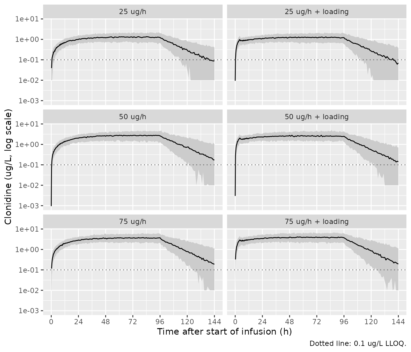
Model-predicted median and 5th-95th percentile clonidine concentrations (with residual error) for the six arms of the Cloesmeijer 2020 study design; analogous to the visual predictive check of Figure 3 (observed data not available).
PKNCA validation
The paper reports no NCA parameters, so PKNCA is used to check internal consistency. Individual predictions are analysed over the 96 h infusion (Cmax, AUC0-96) and over the 48 h washout (terminal half-life). The model is linear in dose, so dose-normalised exposure must match across the 25, 50 and 75 ug/h arms.
conc_nca <- sim_study |>
  filter(!is.na(ipredSim)) |>
  transmute(id, time, conc = ipredSim, treatment = regimen)

conc_obj <- PKNCA::PKNCAconc(conc_nca, conc ~ time | treatment + id)
intervals <- data.frame(
  start = c(0, 96),
  end = c(96, 144),
  cmax = c(TRUE, FALSE),
  auclast = c(TRUE, FALSE),
  half.life = c(FALSE, TRUE)
)
nca_res <- PKNCA::pk.nca(PKNCA::PKNCAdata(conc_obj, intervals = intervals))
#> No dose information provided, calculations requiring dose will return NA.
nca_df <- as.data.frame(nca_res)

nca_summary <- nca_df |>
  filter(PPTESTCD %in% c("cmax", "auclast", "half.life")) |>
  group_by(treatment, PPTESTCD) |>
  summarise(median = median(PPORRES, na.rm = TRUE), .groups = "drop") |>
  tidyr::pivot_wider(names_from = PPTESTCD, values_from = median) |>
  mutate(treatment = factor(treatment, levels = names(study_doses))) |>
  arrange(treatment)

nca_summary |>
  dplyr::rename(
    "Arm" = treatment,
    "Cmax (ug/L)" = cmax,
    "AUC0-96 (h*ug/L)" = auclast,
    "Washout t1/2 (h)" = half.life
  ) |>
knitr::kable(digits = 2, caption = "Median simulated NCA parameters per study arm (individual predictions).")| Arm | AUC0-96 (h*ug/L) | Cmax (ug/L) | Washout t1/2 (h) |
|---|---|---|---|
| 25 ug/h | 106.88 | 1.30 | 11.42 |
| 25 ug/h + loading | 113.79 | 1.34 | 11.28 |
| 50 ug/h | 220.84 | 2.81 | 12.23 |
| 50 ug/h + loading | 230.50 | 2.65 | 11.29 |
| 75 ug/h | 300.83 | 3.72 | 11.09 |
| 75 ug/h + loading | 355.77 | 4.10 | 11.21 |
Two checks are deterministic and use the typical patient (70 kg, no random effects), so they hold exactly on any machine:
- AUC0-96 divided by the maintenance rate is identical for the three arms without a loading dose (linearity);
- the washout half-life that PKNCA fits is close to the terminal
half-life of the two-compartment system,
log(2) / beta, evaluated at the clearance in force halfway through the washout (t = 120 h). Clearance keeps rising during the washout, so the match is approximate rather than exact.
typ_events <- study_events |>
  filter(!loading) |>
  group_by(regimen) |>
  filter(id == min(id)) |>
  ungroup() |>
  mutate(WT = 70)
sim_typ <- rxode2::rxSolve(
  rxode2::zeroRe(mod),
  events = typ_events, keep = c("regimen", "maint_rate"),
  rtol = 1e-10, atol = 1e-12
) |>
  as.data.frame()
#> ℹ parameter labels from comments will be replaced by 'label()'
#> ℹ omega/sigma items treated as zero: 'etalcl', 'etalvc'
#> Warning: multi-subject simulation without without 'omega'

typ_nca <- PKNCA::pk.nca(PKNCA::PKNCAdata(
  PKNCA::PKNCAconc(
    sim_typ |> transmute(id, time, conc = Cc, treatment = regimen),
    conc ~ time | treatment + id
  ),
  intervals = intervals
)) |>
  as.data.frame() |>
  filter(PPTESTCD %in% c("auclast", "half.life")) |>
  select(treatment, PPTESTCD, PPORRES) |>
  tidyr::pivot_wider(names_from = PPTESTCD, values_from = PPORRES) |>
  mutate(maint_rate = as.numeric(sub(" ug/h.*$", "", treatment)))
#> No dose information provided, calculations requiring dose will return NA.

# Terminal half-life of the 2-compartment system at CL(120 h), V1 at 70 kg.
cl120 <- 17.0 * (1 + 0.00213 * 120)
k10 <- cl120 / 124
k12 <- 83.7 / 124
k21 <- 83.7 / 178
beta <- ((k10 + k12 + k21) - sqrt((k10 + k12 + k21)^2 - 4 * k10 * k21)) / 2
t_half_beta <- log(2) / beta

typ_nca |>
  mutate(
    auc_per_rate = auclast / maint_rate,
    beta_half_life = t_half_beta
  ) |>
  dplyr::rename(
    "Arm" = treatment,
    "AUC0-96 (h*ug/L)" = auclast,
    "AUC0-96 / rate (h^2/L)" = auc_per_rate,
    "PKNCA washout t1/2 (h)" = half.life,
    "log(2)/beta at CL(120 h) (h)" = beta_half_life
  ) |>
  select(-maint_rate) |>
knitr::kable(digits = 3, caption = "Typical-patient NCA against the model's closed-form quantities.")| Arm | AUC0-96 (h*ug/L) | PKNCA washout t1/2 (h) | AUC0-96 / rate (h^2/L) | log(2)/beta at CL(120 h) (h) |
|---|---|---|---|---|
| 25 ug/h | 106.750 | 10.676 | 4.27 | 10.728 |
| 50 ug/h | 213.501 | 10.676 | 4.27 | 10.728 |
| 75 ug/h | 320.251 | 10.676 | 4.27 | 10.728 |
auc_per_rate <- typ_nca$auclast / typ_nca$maint_rate
stopifnot(
  nrow(typ_nca) == 3,
  # Linear kinetics: identical to integrator precision.
  max(abs(auc_per_rate / auc_per_rate[1] - 1)) < 1e-6,
  # Approximate: CL rises by about 9% across the 96-144 h washout.
  all(abs(typ_nca$half.life / t_half_beta - 1) < 0.1)
)
Assumptions and deviations
-
Slope units. Table 3 prints the time effect as
“Increase CL per hour 0.213” without a unit. The Discussion states “CL
increased linearly with 0.213%/h from baseline” and that the typical CL
rises from 17 to 20.4 L/h over 4 days;
17 * (1 + 0.00213 * 96) = 20.5 L/hconfirms the percentage reading, so the slope is encoded as 0.00213 per hour. -
Time origin.
tin the model is the time since the start of the clonidine infusion (Methods: “Cov was time in hours”), so the first dose must be att = 0. The effect is not centred and has no plateau; it is valid over the studied treatment span (25-171 h) and extrapolation far beyond it is not supported by the data. - Allometry. Methods Eq 4 mentions an allometric exponent of 0.75 for CL, but Results 3.1.3, the final model of Table 2 (model 9: “time after start infusion on CL + bodyweight on V1”) and the Table 3 units (CL in L/h, V1 in L/70 kg) show that only V1 was weight-scaled in the final model. The model follows the final model.
- Residual error. Table 3 labels the proportional error “(%)” but prints 0.141; both residual terms are read as standard deviations (14.1% and 0.0532 ug/L). The RSE of 4% on the proportional term is at the information floor for an SD with 264 observations, which supports that reading.
-
IIV. Table 3 reports %CV; the variances are
log(CV^2 + 1). - Virtual body weight. Section 2.5 gives the Monte Carlo weight distribution as normal with mean 84 kg and range 53-113 kg but no SD; the vignette uses 15 kg and truncates to the range.
- Loading dose timing. The Figure 1 legend draws the loading dose and the maintenance infusion as consecutive segments, so the study-design simulation gives the 4-h loading infusion first and starts the maintenance rate at 4 h.
-
Screened covariates. Creatinine clearance and
albumin were significant on V1 in forward addition but dropped in
backward elimination; they are recorded in
covariatesDataExcluded. CVVH status was tested and not retained.