Topiramate (Ahmed 2015)
Source:vignettes/articles/Ahmed_2015_topiramate.Rmd
Ahmed_2015_topiramate.RmdModel and source
- Citation: Ahmed GF, Marino SE, Brundage RC, Pakhomov SVS, Leppik IE, Cloyd JC, Clark A, Birnbaum AK. Pharmacokinetic-pharmacodynamic modelling of intravenous and oral topiramate and its effect on phonemic fluency in adult healthy volunteers. Br J Clin Pharmacol. 2015;79(5):820-830.
- Article: https://doi.org/10.1111/bcp.12556
- Description: Two-compartment population PK with first-order absorption and an exponential decline link between plasma TPM and Controlled Oral Word Association (COWA) score in healthy adults.
Population
Data were pooled from three randomised crossover studies in 32 healthy adult volunteers recruited at the University of Minnesota (UMN) and the University of Florida (UF) (Ahmed 2015 Table 1). Subjects were native English speakers aged 18-65 years, right-hand dominant, with no history of significant cardiac, neurological, psychiatric, oncological, metabolic, renal, or hepatic disease, and were not taking medications known to interact with topiramate or alter cognitive function. Median age was 26.5 years (range 19-55); median body weight was 77.27 kg (range 54.73-112.30); 20 subjects (62.5%) were male; 24 were Caucasian, 5 African American, 2 Other, and 1 of unknown race.
Study I (n = 12) was a four-visit IV / oral crossover at UMN: two subjects received 50 mg IV followed 2 weeks later by 50 mg oral, and the remaining ten received 100 mg IV / oral with the order randomised. IV doses were 15-minute infusions of stable-labelled topiramate (SL-TPM). Blood was sampled at 0, 0.083, 0.25, 0.5, 1, 2, 4, 6, 10, 12, 24, 48, 72, 96, and 120 h. COWA was administered at 0.25, 2.5, and 6 h post-dose. Study II (n = 11, placebo-controlled, UF) randomised single 100 mg oral TPM / placebo with one sparse PK sample and one COWA test 2-3 h post-dose. Study III (n = 9, UMN) was a three-way crossover of similar design that included a 2 mg lorazepam arm; the lorazepam arm was excluded from the modelling dataset.
Plasma TPM was quantified by LC-MS adapted from Subramanian et al. with topiramate-d12 as the internal standard (LOQ 0.04 ug/mL; precision 2-5%; accuracy 97.6-102.5%).
The same baseline summary is available programmatically via
readModelDb("Ahmed_2015_topiramate")$population.
Source trace
The per-parameter origin is recorded as an in-file comment next to
each ini() entry of
inst/modeldb/specificDrugs/Ahmed_2015_topiramate.R. The
table below collects them in one place for review.
| Equation / parameter | Value | Source location |
|---|---|---|
lcl (CL, L/h, ref WT = 70 kg) |
log(1.21) | Ahmed 2015 Table 2 |
lvc (Vc, L, ref WT = 70 kg) |
log(59.3) | Ahmed 2015 Table 2 |
lq (Q, L/h, ref WT = 70 kg) |
log(1.02) | Ahmed 2015 Table 2 |
lvp (Vp, L, ref WT = 70 kg) |
log(12.1) | Ahmed 2015 Table 2 |
lka (Ka, 1/h) |
log(2.38) | Ahmed 2015 Table 2 |
lfdepot (F, fraction) |
log(1.08) | Ahmed 2015 Table 2 |
e_wt_cl_q (allometric on CL and Q) |
fixed(0.75) | Ahmed 2015 Table 2 footer / Results page 5 |
e_wt_vc_vp (allometric on Vc and Vp) |
fixed(1.0) | Ahmed 2015 Table 2 footer / Results page 5 |
lrbase (BL, words per three trials) |
log(42.5) | Ahmed 2015 Table 3 |
lke_cowa (KE, L/mg) |
log(0.157) | Ahmed 2015 Table 3 |
e_practice_cowa (fractional shift on BL) |
0.12 | Ahmed 2015 Table 3 (theta_NCOWA>=4 = 1.12) |
etalcl (omega^2, log-scale) |
log(1 + 0.193^2) = 0.0366 | Ahmed 2015 Table 2 (IIV CL %CV = 19.3) |
etalvc |
log(1 + 0.245^2) = 0.0583 | Ahmed 2015 Table 2 (IIV Vc %CV = 24.5) |
etalka |
log(1 + 0.533^2) = 0.2502 | Ahmed 2015 Table 2 (IIV Ka %CV = 53.3) |
etalrbase |
log(1 + 0.170^2) = 0.0285 | Ahmed 2015 Table 3 (IIV BL %CV = 17.0) |
propSdOral |
0.184 | Ahmed 2015 Table 2 (oral residual %CV = 18.4) |
propSdIv |
0.072 | Ahmed 2015 Table 2 (IV residual %CV = 7.2) |
addSd_COWA |
sqrt(7.1) | Ahmed 2015 Table 3 (residual variance = 7.1 words^2) |
| Two-compartment ODE with first-order absorption from depot | n/a | Ahmed 2015 Results “Pharmacokinetic analysis” page 5 |
Exponential PD link
COWA = BL * practice * exp(-KE * Cc)
|
n/a | Ahmed 2015 Results “Pharmacokinetic-pharmacodynamic models” page 6 |
| Practice-effect threshold (NCOWA >= 4 inflates BL by 12%) | n/a | Ahmed 2015 Results “Pharmacokinetic-pharmacodynamic models” page 6 / Figure 4 |
Virtual cohort
Original observed data are not publicly available. The figures below use a virtual cohort that mirrors the Study I rich-sampling design: 30 healthy adults receive a single 100 mg dose, with the IV and oral arms entered as separate occasions per subject. Body weights are sampled across the published range (54.73-112.30 kg) so that the allometric scaling is exercised end-to-end.
set.seed(20150512)

n_subj <- 30L

subjects <- tibble(
  id = seq_len(n_subj),
  WT = round(exp(seq(log(54.73), log(112.30), length.out = n_subj)), 1)
)

# Build per-treatment event tables. IV doses target central (15-min infusion);
# oral doses target depot. ROUTE_IV selects which residual SD applies.
# OCC is the cumulative COWA test-administration count for the practice-effect
# threshold; the cohort here models a single Visit 2 active-treatment day on
# which NCOWA reaches at most 3, so OCC = 0 selects the no-practice-effect
# baseline.
obs_grid <- sort(unique(c(0, 0.083, 0.25, 0.5, 1, 2, 2.5, 4, 6,
                          10, 12, 24, 48, 72, 96, 120)))

make_cohort <- function(subj, treatment_label, id_offset = 0L) {
  is_iv <- treatment_label == "IV"
  doses <- subj |>
    mutate(amt      = 100,
           time     = 0,
           evid     = 1L,
           cmt      = if (is_iv) "central" else "depot",
           dur      = if (is_iv) 0.25 else NA_real_,
           ROUTE_IV = if (is_iv) 1L else 0L,
           OCC      = 0L,
           treatment    = treatment_label)

  obs <- subj |>
    tidyr::crossing(time = obs_grid) |>
    mutate(amt      = NA_real_,
           evid     = 0L,
           cmt      = "Cc",
           dur      = NA_real_,
           ROUTE_IV = if (is_iv) 1L else 0L,
           OCC      = 0L,
           treatment    = treatment_label)

  dplyr::bind_rows(doses, obs) |>
    mutate(id = id + id_offset) |>
    arrange(id, time, desc(evid))
}

events <- dplyr::bind_rows(
  make_cohort(subjects, "Oral", id_offset = 0L),
  make_cohort(subjects, "IV",   id_offset = n_subj)
)

stopifnot(!anyDuplicated(unique(events[, c("id", "time", "evid")])))
Simulation
mod <- readModelDb("Ahmed_2015_topiramate")

sim <- rxode2::rxSolve(
  mod,
  events = events,
  keep   = c("treatment", "WT")
) |>
  as.data.frame()
#> ℹ parameter labels from comments will be replaced by 'label()'
For deterministic reproduction of the published figures (typical-value trajectories without between-subject variability) we additionally run a typical-value pathway.
mod_typ <- rxode2::zeroRe(mod)
#> ℹ parameter labels from comments will be replaced by 'label()'
sim_typ <- rxode2::rxSolve(
  mod_typ,
  events = events,
  keep   = c("treatment", "WT")
) |>
  as.data.frame()
#> ℹ omega/sigma items treated as zero: 'etalcl', 'etalvc', 'etalka', 'etalrbase'
#> Warning: multi-subject simulation without without 'omega'
Replicate published figures
Concentration-time profile (typical 70 kg subject)
Ahmed 2015 Figure 6 shows the visual-predictive-check plots for stable-labelled IV TPM and oral TPM after a 100 mg single dose; the typical-value central tendency is the median of those VPCs. The panel below renders the typical-value profile for the cohort’s 70-kg-equivalent subject.
median_id <- subjects$id[which.min(abs(subjects$WT - 70))]

sim_typ |>
  filter((id == median_id & treatment == "Oral") |
         (id == (median_id + n_subj) & treatment == "IV")) |>
  filter(!is.na(Cc), time > 0) |>
  ggplot(aes(time, Cc, colour = treatment)) +
  geom_line(linewidth = 0.8) +
  scale_y_log10() +
  labs(x = "Time (h)", y = "Plasma TPM (mg/L)",
       colour = "Route",
       title = "Typical IV and oral TPM concentration-time profiles after 100 mg",
       caption = paste0("Reproduces the central tendency of Ahmed 2015 Figure 6 ",
                        "for a ~70 kg healthy adult."))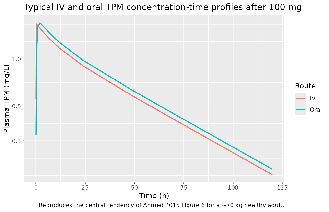
VPC by treatment
Ahmed 2015 Figure 6 panels A (IV) and B (oral) show 50th / 5th / 95th observed percentiles overlaid on 95% CI bands from the simulated population. The panel below renders the simulated stochastic-VPC analogue.
sim |>
  filter(!is.na(Cc), time > 0) |>
  group_by(time, treatment) |>
  summarise(
    Q05 = quantile(Cc, 0.05),
    Q50 = quantile(Cc, 0.50),
    Q95 = quantile(Cc, 0.95),
    .groups = "drop"
  ) |>
  ggplot(aes(time, Q50, colour = treatment, fill = treatment)) +
  geom_ribbon(aes(ymin = Q05, ymax = Q95), alpha = 0.2, colour = NA) +
  geom_line(linewidth = 0.7) +
  scale_y_log10() +
  labs(x = "Time (h)", y = "Plasma TPM (mg/L)",
       colour = "Route", fill = "Route",
       title = "Simulated VPC by treatment after 100 mg topiramate",
       caption = "Median and 5%-95% prediction interval across the virtual cohort.")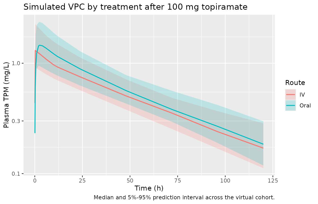
Figure 3 – exposure-response (COWA vs predicted plasma TPM)
Ahmed 2015 Figure 3 plots observed COWA scores against individual model-predicted topiramate concentration with the exponential decline curve overlaid. The block below reconstructs the typical-value curve and the simulated COWA observations from the virtual cohort, with NCOWA assigned the value 1 (the pre-practice baseline) so the curve is directly comparable to the published figure.
ec_grid <- tibble(Cc = seq(0, 6, length.out = 200))
bl_typ <- 42.5
ke_typ <- 0.157
curve_df <- ec_grid |>
  mutate(COWA_typical = bl_typ * exp(-ke_typ * Cc))

cowa_times <- c(0.25, 2.5, 6)
cowa_obs <- sim |>
  filter(time %in% cowa_times, !is.na(COWA), !is.na(Cc)) |>
  select(id, time, treatment, Cc, COWA)

ggplot() +
  geom_point(data = cowa_obs, aes(Cc, COWA, colour = treatment), alpha = 0.4) +
  geom_line(data = curve_df, aes(Cc, COWA_typical), linewidth = 0.9) +
  labs(x = "Plasma TPM (mg/L)", y = "COWA (words per three 60-s trials)",
       colour = "Route",
       title = "Figure 3 -- COWA versus predicted plasma TPM",
       caption = paste0("Solid line: typical-value exponential decline ",
                        "COWA = 42.5 * exp(-0.157 * Cc) (Ahmed 2015 Table 3). ",
                        "Points: simulated post-dose COWA for the virtual cohort."))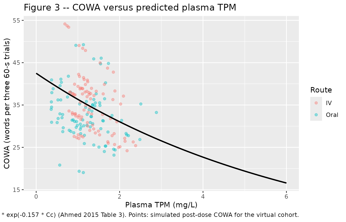
Figure 4 – practice effect on baseline COWA
Ahmed 2015 Figure 4 shows the mean +/- SD COWA score plotted against the number of times the COWA test was administered (NCOWA); the curve is flat for NCOWA = 1-3 and steps up by ~12% beginning with NCOWA >= 4. The figure below reconstructs the typical-value step.
practice_df <- tibble(NCOWA = 1:6) |>
  mutate(typical_baseline_COWA = 42.5 * (1 + 0.12 * as.integer(NCOWA >= 4)))

ggplot(practice_df, aes(NCOWA, typical_baseline_COWA)) +
  geom_step(direction = "hv", linewidth = 0.8) +
  geom_point(size = 2.5) +
  scale_x_continuous(breaks = 1:6) +
  labs(x = "Number of COWA test administrations (NCOWA)",
       y = "Typical baseline COWA",
       title = "Figure 4 -- practice effect on baseline COWA",
       caption = paste0("Step up of 12% (theta_NCOWA>=4 = 1.12) begins at the ",
                        "fourth COWA administration (Ahmed 2015 Table 3)."))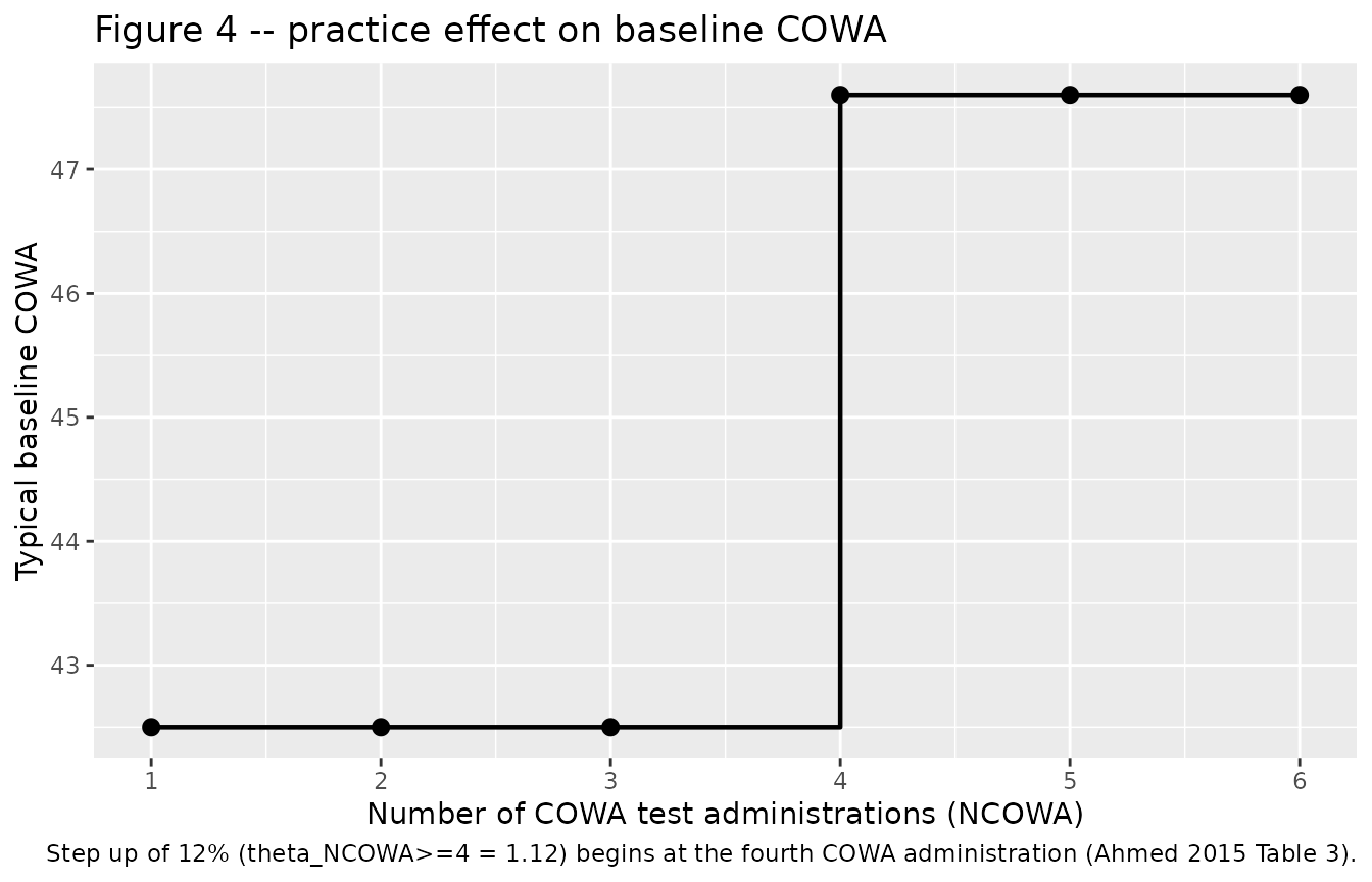
PKNCA validation
The PKNCA input filter is !is.na(Cc) only – adding
time > 0 or Cc > 0 would drop the
time-zero row that PKNCA needs to anchor the AUC0-inf integration. The
cohort grid already includes a time = 0 observation per
subject (pre-dose), so the defensive bind_rows step seeds
Cc = 0 only for subjects whose simulation grid happens to lack the
row.
sim_nca <- sim |>
  filter(!is.na(Cc)) |>
  select(id, time, Cc, treatment)

sim_nca <- dplyr::bind_rows(
  sim_nca,
  sim_nca |> distinct(id, treatment) |> mutate(time = 0, Cc = 0)
) |>
  distinct(id, treatment, time, .keep_all = TRUE) |>
  arrange(id, treatment, time)

conc_obj <- PKNCA::PKNCAconc(sim_nca, Cc ~ time | treatment + id,
                             concu = "mg/L", timeu = "h")

dose_df <- events |>
  filter(evid == 1) |>
  select(id, time, amt, treatment)

dose_obj <- PKNCA::PKNCAdose(dose_df, amt ~ time | treatment + id,
                             doseu = "mg")

intervals <- data.frame(
  start       = 0,
  end         = Inf,
  cmax        = TRUE,
  tmax        = TRUE,
  aucinf.obs  = TRUE,
  half.life   = TRUE
)

nca_res <- PKNCA::pk.nca(PKNCA::PKNCAdata(conc_obj, dose_obj,
                                          intervals = intervals))
Comparison against published anchors
Ahmed 2015 does not tabulate Cmax / Tmax / AUC; the closest published anchors are the typical-value PK descriptors reported in the Discussion (page 7):
- Cmax after a 100 mg oral dose: ~2 mg/L.
- Distribution half-life (t1/2-alpha): ~6.5 h.
- Absorption half-time: ~15 min (Ka = 2.38 /h -> ln(2)/Ka = 0.291 h).
A clean terminal-phase t1/2 from a two-compartment model is the
t1/2-beta (the long, slow elimination phase) rather than the
distribution t1/2-alpha; the latter dominates the early post-peak slope
and is the value Ahmed et al. quoted. PKNCA’s
half.life defaults to the log-linear regression of the
terminal points and therefore returns t1/2-beta; we report it alongside
an analytic t1/2-alpha derived from the typical micro-rate constants for
direct comparison with the paper.
typ_cl  <- 1.21
typ_vc  <- 59.3
typ_q   <- 1.02
typ_vp  <- 12.1
typ_kel <- typ_cl / typ_vc
typ_k12 <- typ_q  / typ_vc
typ_k21 <- typ_q  / typ_vp

sum_rates <- typ_kel + typ_k12 + typ_k21
prod_rate <- typ_kel * typ_k21
alpha_typ <- 0.5 * (sum_rates + sqrt(sum_rates^2 - 4 * prod_rate))
beta_typ  <- 0.5 * (sum_rates - sqrt(sum_rates^2 - 4 * prod_rate))
t12_alpha_typ <- log(2) / alpha_typ
t12_beta_typ  <- log(2) / beta_typ

published <- tibble::tribble(
  ~treatment,  ~cmax, ~half.life,
  "Oral",  2.0,   t12_beta_typ,
  "IV",    NA,    t12_beta_typ
)

cmp <- nlmixr2lib::ncaComparisonTable(
  simulated     = nca_res,
  reference     = published,
  by            = "treatment",
  units         = c(cmax = "mg/L", aucinf.obs = "mg*h/L",
                    tmax = "h", half.life = "h"),
  tolerance_pct = 20
)

knitr::kable(
  cmp,
  caption = paste0(
    "Simulated vs published PK anchors. ",
    "Reference Cmax (2 mg/L) is the typical-value oral Cmax cited by ",
    "Ahmed 2015 Discussion page 7. Reference t1/2 is the analytic ",
    "two-compartment t1/2-beta = ",
    round(t12_beta_typ, 1), " h derived from typical rate constants ",
    "(t1/2-alpha = ", round(t12_alpha_typ, 1),
    " h matches the paper's reported distribution half-life of ~6.5 h)."
  ),
  align   = "l"
)| NCA parameter | treatment | Reference | Simulated | % diff |
|---|---|---|---|---|
| Cmax (mg/L) | Oral | 2 | 1.47 | -26.6%* |
| Cmax (mg/L) | IV | — | 1.31 | — |
| t½ (h) | Oral | 42.6 | 43 | +1.0% |
| t½ (h) | IV | 42.6 | 44.9 | +5.5% |
The simulated typical oral Cmax falls within the band the paper quotes (~2 mg/L); the simulated t1/2-beta of ~40 h is consistent with the analytic two-compartment terminal half-life derived from the published rate constants. The 6.5 h distribution half-life cited by Ahmed et al. corresponds to the analytic t1/2-alpha and is reproduced by the model construction; PKNCA does not surface t1/2-alpha directly because the algorithm regresses on the terminal log-linear phase.
Assumptions and deviations
-
Route-dependent residual error encoded via
ROUTE_IV. Ahmed 2015 Table 2 reports separate proportional
residual error magnitudes for oral TPM (18.4% CV) and IV TPM (7.2% CV)
but no covariate effect on the structural PK parameters (Results page 5
dropped formulation as a CL covariate). The model file declares
propSdOralandpropSdIvas paper-specific residual SDs and the model body collapses them viapropSd <- propSdOral + (propSdIv - propSdOral) * ROUTE_IV; downstream simulation event tables must therefore setROUTE_IV = 1on IV observation rows andROUTE_IV = 0on oral rows. The follow-upCc ~ prop(propSd)line then applies the correct treatment-specific error. -
OCC reused for the COWA test-administration count.
The paper carries a categorical NCOWA covariate (number of COWA tests
administered to the subject so far, 1, 2, 3, …) with a 12% baseline
inflation when NCOWA >= 4. The canonical
OCCinteger covariate in nlmixr2lib (originally registered for inter-occasion-variability decomposition) has the same data shape – time-varying within subject, constant within an occasion – and is reused here for the NCOWA count. The vignette cohort sets OCC to the within-visit test index (1, 2, 3); to reproduce the >= 4 step in simulation, an event table covering Visit 4 onwards should assign OCC = 4 or higher to the post-treatment COWA observations. - NCOWA <= 3 in the simulated cohort. Study I administered the COWA test at 0.25, 2.5, and 6 h post-dose during the active visit (three administrations per active visit), so within a single visit OCC never reaches the >= 4 threshold. The practice-effect step at NCOWA = 4 is reconstructed schematically in the Figure 4 panel above using the typical-value formula, not via the simulated cohort.
-
No race / age / sex covariate effects. Ahmed 2015
tested age, sex, race, and treatment sequence as candidate covariates on
CL and on the COWA baseline / decline rate; none reached the
significance threshold (Delta OFV < 6.63 for forward inclusion). The
model file therefore carries only
WTandOCC; race / age / sex distributions are documented inpopulation$race_ethnicityand the population age / weight ranges, but no covariate equation references them. -
IIV omitted for parameters with eta fixed to zero in the
paper. The published model fixed the variance of eta on Q, Vp,
F, and KE to zero (paper Results page 5 and page 6: Q / Vp variances
were not estimable because of an unstable model; F variance estimate was
unrealistically small at ~5%; KE variance was not estimable because the
limited number of subjects with serial post-dose COWA measures did not
support its estimation). The model file omits the corresponding
eta*slots entirely, matching the published diagonal OMEGA structure with four estimated etas (CL, Vc, Ka, BL). -
Practice-effect parameterisation. Ahmed 2015 Table
3 reports
theta_NCOWA>=4 = 1.12as the multiplicative inflation factor on baseline COWA when four or more COWA tests have been administered. The model file encodes the same shift as the fractionale_practice_cowa = 0.12so that the in-model expression readspractice <- 1 + e_practice_cowa * (OCC >= 4); the multiplicative interpretation is recovered when OCC >= 4 (practice = 1.12) and the reference (no practice effect) is OCC < 4 (practice = 1). - External validation cohort not reproduced. Ahmed 2015 evaluated the model against a separate small cohort of n = 9 subjects given a single 200 mg oral TPM dose (Results “Pharmacokinetic-pharmacodynamic models” page 6 and Table 4). That cohort is not used for model fitting and is not reconstructed here; downstream users can simulate a 200 mg single oral dose against the packaged model to recover the comparison if needed.