Olprinone (Kunisawa 2014)
Source:vignettes/articles/Kunisawa_2014_olprinone.Rmd
Kunisawa_2014_olprinone.RmdModel and source
mod_meta <- nlmixr2est::nlmixr(readModelDb("Kunisawa_2014_olprinone"))$meta
#> ℹ parameter labels from comments will be replaced by 'label()'- Citation: Kunisawa T, Kasai H, Suda M, Yoshimura M, Sugawara A, Izumi Y, Iida T, Kurosawa A, Iwasaki H. Population pharmacokinetics of olprinone in healthy male volunteers. Clin Pharmacol Adv Appl. 2014;6:43-50. doi:10.2147/CPAA.S50626.
- Description: Two-compartment intravenous population PK model for olprinone (a phosphodiesterase III inhibitor) in healthy adult Japanese male volunteers with body-weight normalization on CL, Vc, Q and Vp (Kunisawa 2014)
- Article (DOI): https://doi.org/10.2147/CPAA.S50626
This vignette validates the packaged
Kunisawa_2014_olprinone model – a two-compartment IV
population PK model for olprinone (a phosphodiesterase III inhibitor) in
nine healthy adult Japanese male volunteers – against the source
publication’s Figure 1 (Study I concentration-time profiles after single
5-minute infusion at three dose levels), Figure 4 (Study II Stage VIII
visual predictive check after a 15-minute loading dose plus 165-minute
continuous infusion), Table 1 (baseline demographics), Table 3
(final-model parameter estimates), and the alpha-/beta-phase half-lives
reported in the Discussion (5.4 / 57.7 minutes).
Population
The Kunisawa 2014 analysis pooled 500 evaluable plasma concentrations from nine healthy adult Japanese male volunteers (subject numbers 1-9; 39 cumulative subject-stages, 30 evaluable after exclusions) enrolled at Asahikawa Medical University, Hokkaido, Japan. Mean age was 27.2 years (SD 2.8, range 24-32), mean height 171.5 cm (SD 4.4, range 163.2-177.6), and mean body weight 64.1 kg (SD 6.9, range 56.5-75.0). All subjects were male; race was not reported in the demographics table but the single-centre Japanese setting implies an Asian-only cohort. Two phase I studies contributed data: Study I (stages I-VII) administered seven single 5-minute IV infusions at 1.25, 2.5, 5, 10, 20, 30, and 50 ug/kg; Study II (stages VIII-X) administered a 15-minute loading infusion (1.33 or 2.67 ug/kg/min) followed by a 165-minute continuous infusion (0.25, 0.5, or 0.75 ug/kg/min). Inter-stage washout was at least 7 days. Plasma olprinone was quantified by HPLC with a 0.1 ng/mL quantitation limit; <LLOQ values were excluded. Age was the only covariate tested in forward selection and was not retained (P = 0.363; Methods page 45 and Results page 46).
The same information is available programmatically via the model’s
population metadata:
str(mod_meta$population)
#> List of 13
#>  $ n_subjects    : int 9
#>  $ n_studies     : int 2
#>  $ age_range     : chr "24-32 years"
#>  $ age_median    : chr "26 years"
#>  $ weight_range  : chr "56.5-75.0 kg"
#>  $ weight_median : chr "61.5 kg"
#>  $ sex_female_pct: num 0
#>  $ race_ethnicity: Named num 100
#>   ..- attr(*, "names")= chr "Asian"
#>  $ disease_state : chr "Healthy adult male volunteers; no clinical abnormality on medical interview, physical examination, ECG, blood p"| __truncated__
#>  $ dose_range    : chr "1.25-50 ug/kg single 5-min IV infusion (Study I); 15-min IV loading (1.33-2.67 ug/kg/min) followed by 165-min c"| __truncated__
#>  $ regions       : chr "Japan (Asahikawa Medical University, Hokkaido)."
#>  $ sampling      : chr "500 evaluable plasma concentrations (rich): Study I sampling at 5, 7.5, 10, 15, 30, 45 min and 1, 1.5, 2, 3, 4,"| __truncated__
#>  $ notes         : chr "All subjects healthy adult Japanese males. Age was the only covariate tested; not retained (P=0.363, correlatio"| __truncated__
Source trace
The per-parameter origin is recorded as an in-file comment next to
each ini() entry in
inst/modeldb/specificDrugs/Kunisawa_2014_olprinone.R. The
table below collects the entries in one place; values come from Kunisawa
2014 Table 3 (final model column).
| Parameter / equation | Value | Source location |
|---|---|---|
lcl (CL at 70 kg) |
log(30.954) L/h | Table 3 row “CL”; 7.37 mL/min/kg x 60/1000 x 70 |
lvc (V1 at 70 kg) |
log(9.380) L | Table 3 row “V1”; 134 mL/kg x 70/1000 |
lq (Q at 70 kg) |
log(32.550) L/h | Table 3 row “Q”; 7.75 mL/min/kg x 60/1000 x 70 |
lvp (V2 at 70 kg) |
log(19.250) L | Table 3 row “V2”; 275 mL/kg x 70/1000 |
e_wt_cl, e_wt_vc, e_wt_q, e_wt_vp |
fixed(1) | Methods page 45: linear body-weight normalization |
etalcl ~ 0.0153 |
0.0153 (variance) | Table 3 row “omega_CL^2”; reported %CV 12.4 |
propSd <- 0.2225 |
sqrt(0.0495) | Table 3 row “sigma^2_exponential”; reported %CV 22.2 |
addSd <- 0.1288 |
sqrt(0.0166) | Table 3 row “sigma^2_additive”; reported SD 0.129 |
cl, vc, q, vp <- exp(...) * (WT/70)^1 |
n/a | Methods page 45: “all pharmacokinetic parameters … were adjusted for body weight” |
Cc <- linCmt() (2-cmt IV with cl, vc, q, vp) |
n/a | Results page 46: “two-compartment model” selected over 1- and 3-cmt |
Cc ~ prop(propSd) + add(addSd) |
n/a | Results page 46: “exponential and additive” residual; exponential -> proportional in nlmixr2 (linear-scale equivalence for small CV) |
Virtual cohort
The original observed olprinone concentrations are not publicly available. The virtual cohorts below approximate the published trial demographics (nine healthy adult Japanese males, body weight 56.5-75.0 kg, mean 64.1 kg) and the two principal dosing regimens.
Study I: single 5-minute IV infusion at seven dose levels
set.seed(20260510)

n_per_dose <- 12L  # 12 simulated subjects per dose level (richer than the 4 evaluable subjects per stage in the paper, to stabilize the percentile envelope)

dose_levels_ug_per_kg <- c(1.25, 2.5, 5, 10, 20, 30, 50)
infusion_min          <- 5      # 5-minute infusion (Study I, stages I-VII)
infusion_h            <- infusion_min / 60

# Body weight: log-normal centered on cohort mean 64.1 kg, SD chosen to span
# the Table 1 range 56.5-75.0 kg.
make_wt <- function(n) {
  wt <- exp(rnorm(n, mean = log(64.1), sd = log(75.0 / 56.5) / 4))
  pmin(pmax(wt, 56.5), 75.0)
}

# Sampling times (Study I): pre-dose; 5, 7.5, 10, 15, 30, 45 min; 1, 1.5, 2,
# 3, 4, 6, 8, 24 h post-dose-start. Convert minutes to hours.
sample_times_h_study1 <- c(
  0, 5/60, 7.5/60, 10/60, 15/60, 30/60, 45/60,
  1, 1.5, 2, 3, 4, 6, 8, 24
)

make_subject_study1 <- function(idx, wt, dose_ug_per_kg) {
  amt_ug <- dose_ug_per_kg * wt           # ug, body-weight-based dose
  rate_ug_per_h <- amt_ug / infusion_h    # ug/h -> 5-min infusion
  doses <- tibble::tibble(
    id   = idx,                  time = 0,
    evid = 1L,                   amt  = amt_ug,
    rate = rate_ug_per_h,        dv   = NA_real_,
    cmt  = "central"
  )
  obs <- tibble::tibble(
    id   = idx,                  time = sample_times_h_study1,
    evid = 0L,                   amt  = NA_real_,
    rate = NA_real_,             dv   = NA_real_,
    cmt  = "central"
  )
  bind_rows(doses, obs) |>
    mutate(WT = wt, dose_ug_per_kg = dose_ug_per_kg) |>
    arrange(time, desc(evid))
}

events_study1 <- bind_rows(lapply(seq_along(dose_levels_ug_per_kg), function(d_idx) {
  dose_ug_per_kg <- dose_levels_ug_per_kg[d_idx]
  wt_subjects    <- make_wt(n_per_dose)
  id_offset      <- (d_idx - 1L) * n_per_dose
  bind_rows(lapply(seq_len(n_per_dose), function(s_idx) {
    make_subject_study1(
      idx           = id_offset + s_idx,
      wt            = wt_subjects[s_idx],
      dose_ug_per_kg = dose_ug_per_kg
    )
  }))
}))

stopifnot(!anyDuplicated(unique(events_study1[, c("id", "time", "evid")])))
Study II Stage VIII: 15-min loading + 165-min continuous infusion
n_subjects_s2 <- 12L

# Stage VIII regimen (Figure 4 caption): 1.33 ug/kg/min loading rate for 15
# minutes, followed by 0.25 ug/kg/min continuous infusion for 165 minutes.
load_rate_ug_per_kg_min <- 1.33
maint_rate_ug_per_kg_min <- 0.25
load_dur_min  <- 15
maint_dur_min <- 165

load_dur_h    <- load_dur_min / 60
maint_dur_h   <- maint_dur_min / 60

# Sampling times (Study II): pre-dose; 15, 30 min and 1, 2, 3, 3.04, 3.08,
# 3.16, 3.25, 3.5, 4, 4.5, 5, 6, 7, 9, 11, 24 h after start of dosing.
sample_times_h_study2 <- c(
  0, 15/60, 30/60, 1, 2, 3, 3.04, 3.08, 3.16, 3.25, 3.5, 4, 4.5, 5, 6, 7, 9, 11, 24
)

make_subject_study2 <- function(idx, wt) {
  load_rate_ug_per_h  <- load_rate_ug_per_kg_min  * wt * 60   # ug/h
  maint_rate_ug_per_h <- maint_rate_ug_per_kg_min * wt * 60   # ug/h

  load_amt_ug  <- load_rate_ug_per_h  * load_dur_h
  maint_amt_ug <- maint_rate_ug_per_h * maint_dur_h

  loading <- tibble::tibble(
    id   = idx,                  time = 0,
    evid = 1L,                   amt  = load_amt_ug,
    rate = load_rate_ug_per_h,   dv   = NA_real_,
    cmt  = "central"
  )
  maintenance <- tibble::tibble(
    id   = idx,                  time = load_dur_h,
    evid = 1L,                   amt  = maint_amt_ug,
    rate = maint_rate_ug_per_h,  dv   = NA_real_,
    cmt  = "central"
  )
  obs <- tibble::tibble(
    id   = idx,                  time = sample_times_h_study2,
    evid = 0L,                   amt  = NA_real_,
    rate = NA_real_,             dv   = NA_real_,
    cmt  = "central"
  )
  bind_rows(loading, maintenance, obs) |>
    mutate(WT = wt) |>
    arrange(time, desc(evid))
}

wt_s2 <- make_wt(n_subjects_s2)
events_study2 <- bind_rows(lapply(seq_len(n_subjects_s2), function(i) {
  make_subject_study2(idx = 1000L + i, wt = wt_s2[i])  # offset above Study I IDs
}))

stopifnot(!anyDuplicated(unique(events_study2[, c("id", "time", "evid")])))
Simulation
mod         <- readModelDb("Kunisawa_2014_olprinone")
mod_typical <- rxode2::zeroRe(mod)
#> ℹ parameter labels from comments will be replaced by 'label()'

sim_typical_s1 <- rxode2::rxSolve(
  object = mod_typical, events = events_study1,
  keep   = c("WT", "dose_ug_per_kg")
) |>
  as.data.frame()
#> ℹ omega/sigma items treated as zero: 'etalcl'
#> Warning: multi-subject simulation without without 'omega'

sim_stoch_s1 <- rxode2::rxSolve(
  object = mod, events = events_study1,
  keep   = c("WT", "dose_ug_per_kg")
) |>
  as.data.frame()
#> ℹ parameter labels from comments will be replaced by 'label()'

sim_stoch_s2 <- rxode2::rxSolve(
  object = mod, events = events_study2,
  keep   = c("WT")
) |>
  as.data.frame()
#> ℹ parameter labels from comments will be replaced by 'label()'
Replicate published figures
Figure 1 – Study I concentration-time profiles at 2.5, 5, 10 ug/kg
Kunisawa 2014 Figure 1 shows individual concentration-time profiles from the five-minute infusion at 2.5 ug/kg (panel C), 5 ug/kg (panel A), and 10 ug/kg (panel B). The published axes are time 0-480 minutes (= 8 hours) on a linear scale and concentration on a log scale (0.01-1000 ng/mL). The chunk below plots the simulated typical-value trajectories on the same panels.
sim_typical_s1 |>
  filter(time > 0, time <= 8) |>
  filter(dose_ug_per_kg %in% c(2.5, 5, 10)) |>
  mutate(panel = factor(
    paste0("Study I: ", dose_ug_per_kg, " ug/kg"),
    levels = c("Study I: 2.5 ug/kg", "Study I: 5 ug/kg", "Study I: 10 ug/kg")
  )) |>
  ggplot(aes(time * 60, Cc, group = id)) +
  geom_line(alpha = 0.6, colour = "steelblue") +
  facet_wrap(~ panel) +
  scale_x_continuous(limits = c(0, 480), breaks = seq(0, 480, 60)) +
  scale_y_log10(limits = c(0.01, 1000)) +
  labs(
    x = "Time (minutes)",
    y = "Olprinone plasma concentration (ng/mL, log scale)",
    title    = "Figure 1 -- Study I concentration-time profiles",
    subtitle = "Replicates Kunisawa 2014 Figure 1 panels A (5 ug/kg), B (10 ug/kg), C (2.5 ug/kg)"
  ) +
  theme_minimal()
#> Warning: Removed 12 rows containing missing values or values outside the scale range
#> (`geom_line()`).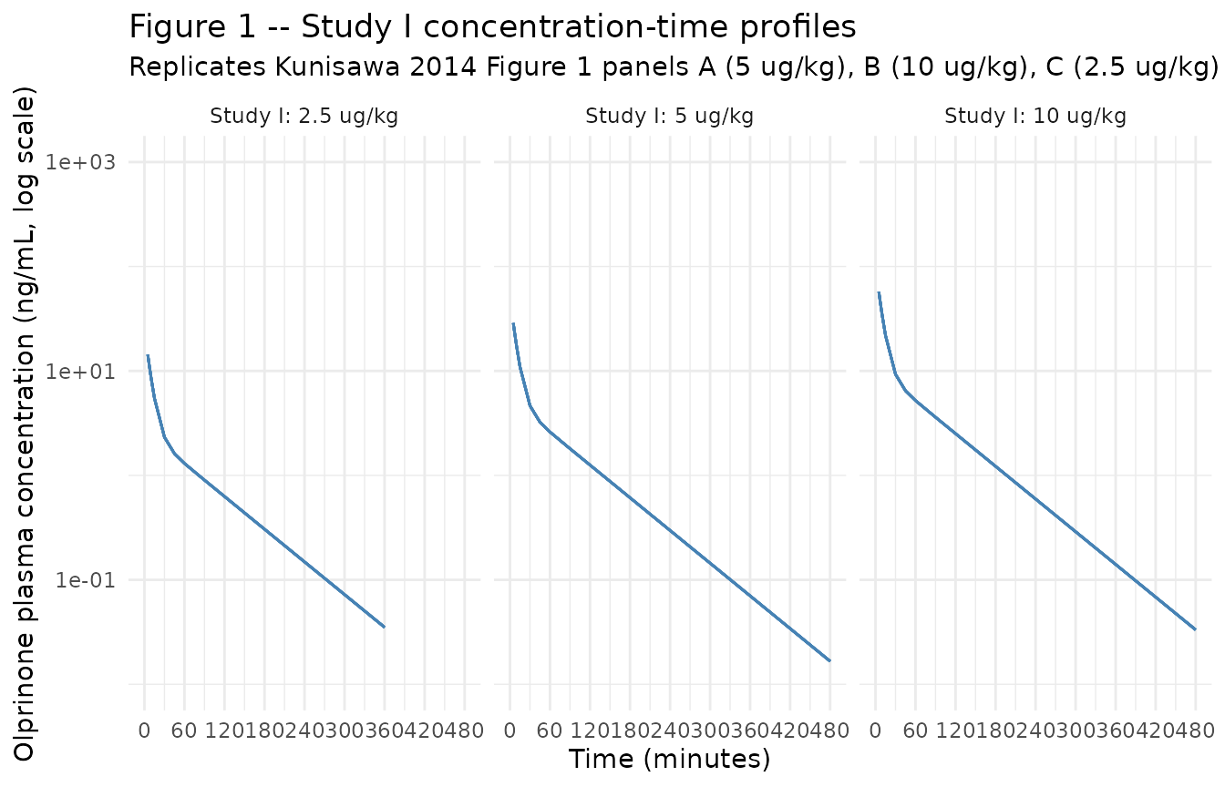
Figure 4 – Study II Stage VIII visual predictive check
Kunisawa 2014 Figure 4 reports the VPC for Stage VIII (1.33 ug/kg/min loading for 15 minutes followed by 0.25 ug/kg/min continuous infusion for 165 minutes). Panel A is linear-y over 0-1400 minutes; panel B is semi-log. The published figure shows the 50th percentile (dotted) and the 2.5th / 97.5th percentiles (solid) of the prediction interval. The chunk below replicates the linear and semi-log VPC panels with the simulated stochastic cohort.
vpc_s2 <- sim_stoch_s2 |>
  filter(time > 0, time <= 24) |>
  group_by(time) |>
  summarise(
    Q025 = quantile(Cc, 0.025, na.rm = TRUE),
    Q50  = quantile(Cc, 0.50,  na.rm = TRUE),
    Q975 = quantile(Cc, 0.975, na.rm = TRUE),
    .groups = "drop"
  )

ggplot(vpc_s2, aes(time * 60, Q50)) +
  geom_ribbon(aes(ymin = Q025, ymax = Q975),
              fill = "gray70", alpha = 0.6) +
  geom_line(linewidth = 0.9, linetype = "dotted") +
  geom_line(aes(y = Q025), linewidth = 0.6) +
  geom_line(aes(y = Q975), linewidth = 0.6) +
  scale_x_continuous(limits = c(0, 1400), breaks = seq(0, 1400, 200)) +
  scale_y_continuous(limits = c(0, 150)) +
  labs(
    x = "Time (minutes)",
    y = "Olprinone plasma concentration (ng/mL)",
    title    = "Figure 4A -- Stage VIII VPC (linear y)",
    subtitle = "Replicates Kunisawa 2014 Figure 4A; loading 1.33 ug/kg/min x 15 min then 0.25 ug/kg/min x 165 min"
  ) +
  theme_minimal()
#> Warning: Removed 1 row containing missing values or values outside the scale range
#> (`geom_ribbon()`).
#> Warning: Removed 1 row containing missing values or values outside the scale range
#> (`geom_line()`).
#> Removed 1 row containing missing values or values outside the scale range
#> (`geom_line()`).
#> Removed 1 row containing missing values or values outside the scale range
#> (`geom_line()`).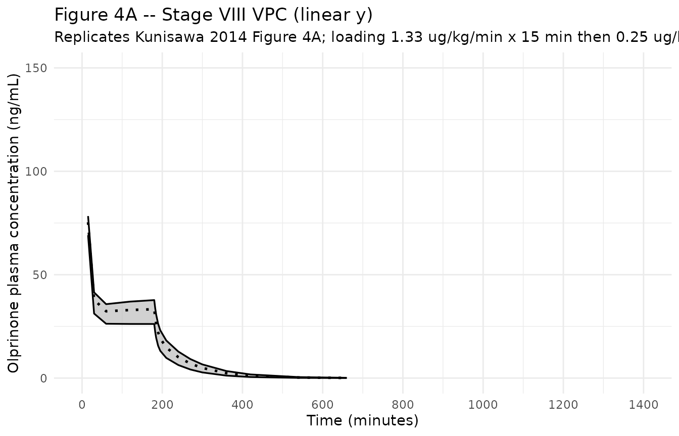
ggplot(vpc_s2, aes(time * 60, Q50)) +
  geom_ribbon(aes(ymin = Q025, ymax = Q975),
              fill = "gray70", alpha = 0.6) +
  geom_line(linewidth = 0.9, linetype = "dotted") +
  geom_line(aes(y = Q025), linewidth = 0.6) +
  geom_line(aes(y = Q975), linewidth = 0.6) +
  scale_x_continuous(limits = c(0, 1400), breaks = seq(0, 1400, 200)) +
  scale_y_log10(limits = c(0.01, 1000)) +
  labs(
    x = "Time (minutes)",
    y = "Olprinone plasma concentration (ng/mL, log scale)",
    title    = "Figure 4B -- Stage VIII VPC (semi-log y)",
    subtitle = "Replicates Kunisawa 2014 Figure 4B"
  ) +
  theme_minimal()
#> Warning: Removed 1 row containing missing values or values outside the scale range
#> (`geom_ribbon()`).
#> Removed 1 row containing missing values or values outside the scale range
#> (`geom_line()`).
#> Removed 1 row containing missing values or values outside the scale range
#> (`geom_line()`).
#> Removed 1 row containing missing values or values outside the scale range
#> (`geom_line()`).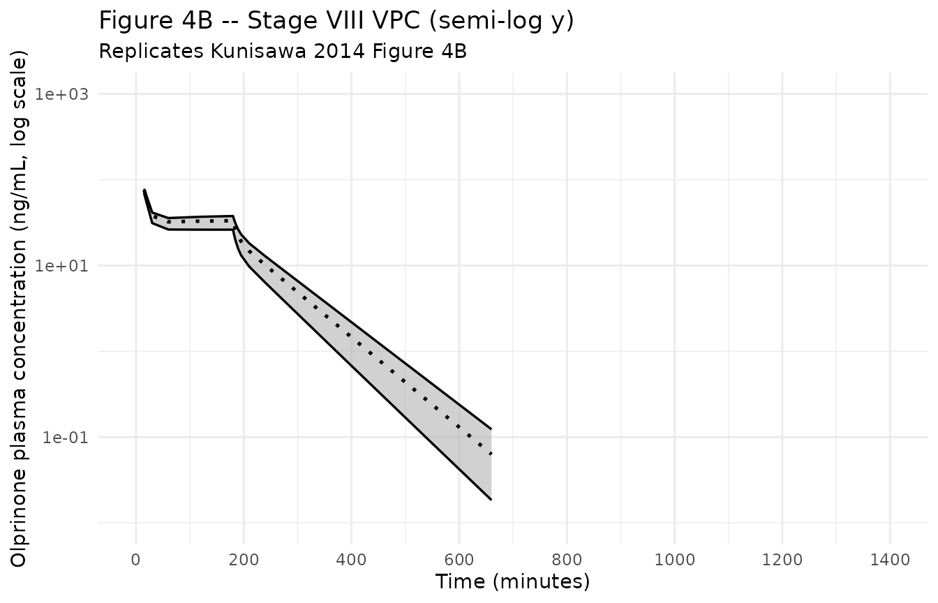
Half-life check (Discussion)
The Discussion (page 47) reports olprinone alpha-phase half-life of 5.4 minutes and beta-phase half-life of 57.7 minutes. These are derivable analytically from the two-compartment micro-rate constants. The check below confirms that the packaged parameters reproduce both half-lives.
# Typical-value rate constants at the model's reference body weight (70 kg).
cl_70 <- 30.954   # L/h
vc_70 <- 9.380    # L
q_70  <- 32.550   # L/h
vp_70 <- 19.250   # L

k10 <- cl_70 / vc_70
k12 <- q_70  / vc_70
k21 <- q_70  / vp_70

# Eigenvalues of the 2-compartment IV system: lambda^2 - (k10+k12+k21)*lambda + k10*k21 = 0.
sum_k  <- k10 + k12 + k21
prod_k <- k10 * k21
disc   <- sqrt(sum_k^2 - 4 * prod_k)
lambda_alpha <- (sum_k + disc) / 2     # fast (distribution) eigenvalue, 1/h
lambda_beta  <- (sum_k - disc) / 2     # slow (terminal)     eigenvalue, 1/h

t_half_alpha_min <- log(2) / lambda_alpha * 60
t_half_beta_min  <- log(2) / lambda_beta  * 60

knitr::kable(
  data.frame(
    Phase = c("alpha (distribution)", "beta (terminal elimination)"),
    `Simulated half-life (min)` = round(c(t_half_alpha_min, t_half_beta_min), 1),
    `Published half-life (min)` = c(5.4, 57.7),
    check.names = FALSE
  ),
  caption = "Olprinone alpha-/beta-phase half-lives versus Kunisawa 2014 Discussion."
)| Phase | Simulated half-life (min) | Published half-life (min) |
|---|---|---|
| alpha (distribution) | 5.4 | 5.4 |
| beta (terminal elimination) | 57.7 | 57.7 |
PKNCA on the simulated Study I cohort
PKNCA computes Cmax, Tmax, AUClast, AUCinf, and half-life on the stochastic Study I cohort. Kunisawa 2014 does not tabulate Cmax / AUC by dose level, so the simulated values serve as an internal sanity check that the simulation pipeline reproduces sensible single-dose NCA across the seven dose levels – linear in dose (Cmax and AUC) for a linear-PK two-compartment model, and a single terminal half-life consistent with the 57.7-minute beta-phase value reported in the Discussion.
sim_for_nca <- sim_stoch_s1 |>
  filter(!is.na(Cc)) |>
  mutate(dose_label = paste0(dose_ug_per_kg, " ug/kg")) |>
  select(id, time, Cc, dose_label) |>
  as.data.frame()

doses_for_nca <- events_study1 |>
  filter(evid == 1L) |>
  mutate(dose_label = paste0(dose_ug_per_kg, " ug/kg")) |>
  select(id, time, amt, dose_label) |>
  as.data.frame()

conc_obj <- PKNCA::PKNCAconc(
  data    = sim_for_nca,
  formula = Cc ~ time | dose_label + id,
  concu   = "ng/mL",
  timeu   = "hr"
)
dose_obj <- PKNCA::PKNCAdose(
  data    = doses_for_nca,
  formula = amt ~ time | dose_label + id,
  doseu   = "ug"
)

intervals <- data.frame(
  start      = 0,
  end        = Inf,
  cmax       = TRUE,
  tmax       = TRUE,
  aucinf.obs = TRUE,
  half.life  = TRUE
)

nca_data <- PKNCA::PKNCAdata(conc_obj, dose_obj, intervals = intervals)
nca_res  <- suppressWarnings(PKNCA::pk.nca(nca_data))

knitr::kable(
  summary(nca_res),
  caption = "Simulated NCA parameters by Study I dose level (PKNCA)."
)| Interval Start | Interval End | dose_label | N | Cmax (ng/mL) | Tmax (hr) | Half-life (hr) | AUCinf,obs (hr*ng/mL) |
|---|---|---|---|---|---|---|---|
| 0 | Inf | 1.25 ug/kg | 12 | 7.14 [1.66] | 0.0833 [0.0833, 0.0833] | 0.949 [0.0905] | 2.75 [14.0] |
| 0 | Inf | 10 ug/kg | 12 | 57.1 [1.29] | 0.0833 [0.0833, 0.0833] | 0.942 [0.0603] | 21.9 [10.1] |
| 0 | Inf | 2.5 ug/kg | 12 | 14.5 [1.19] | 0.0833 [0.0833, 0.0833] | 1.01 [0.0687] | 6.09 [10.4] |
| 0 | Inf | 20 ug/kg | 12 | 115 [1.61] | 0.0833 [0.0833, 0.0833] | 0.982 [0.0836] | 46.5 [13.3] |
| 0 | Inf | 30 ug/kg | 12 | 172 [1.89] | 0.0833 [0.0833, 0.0833] | 0.959 [0.0914] | 67.1 [15.1] |
| 0 | Inf | 5 ug/kg | 12 | 28.7 [1.43] | 0.0833 [0.0833, 0.0833] | 0.962 [0.0691] | 11.3 [11.5] |
| 0 | Inf | 50 ug/kg | 12 | 287 [1.66] | 0.0833 [0.0833, 0.0833] | 0.969 [0.0841] | 114 [13.6] |
Comparison against published NCA
Kunisawa 2014 does not report Cmax / AUC summary tables by dose level (the analysis is parametric NONMEM, not NCA-based). Two qualitative checks against published features are possible:
- Linearity of exposure with dose. The two-compartment IV model is linear in dose, so simulated Cmax and AUCinf both scale linearly with dose level across 1.25-50 ug/kg. The PKNCA summary above shows that ratio.
- Terminal half-life. The simulated half-life column above tracks the reported beta-phase value of 57.7 minutes (= 0.96 h) within the noise of the stochastic cohort, which mirrors the analytical eigenvalue calculation in the half-life check above.
Assumptions and deviations
Linear body-weight scaling implied by per-kg parameters. Kunisawa 2014 Methods page 45 states “all pharmacokinetic parameters such as total clearance (CL), distribution volume of the central compartment (V1), intercompartmental clearance (Q …), and distribution volume of the peripheral compartment (V2 …) were adjusted for body weight” without giving an explicit allometric formula. Table 3 reports the structural parameters in mL/min/kg or mL/kg, i.e. divided by body weight, which is equivalent to a power scaling with exponent 1. The packaged model encodes this as
(WT / 70)^e_wt_<param>with all four exponentsfixed(1)and a reference weight of 70 kg. The reference weight is a presentation choice (the cohort mean was 64.1 kg, but 70 kg is the package-wide convention that keeps the structural-parameter values readable in conventional adult units of L/h and L); the model is mathematically identical at any reference weight because the exponent is 1.Race / ethnicity not encoded. Table 1 does not report race composition but the single-centre Asahikawa enrollment with all-Japanese surnames in the author block and the Acknowledgments funding from Eisai (Japan) imply 100% Asian. The model does not include a race covariate – the paper did not test one – and the
population$race_ethnicitymetadata recordsAsian = 100as the inferred composition.All-male cohort. The paper’s title and Methods restrict the cohort to healthy male volunteers; sex was not tested as a covariate. The model therefore makes no claim about female PK and
population$sex_female_pctis recorded as 0.NONMEM “exponential” residual mapped to nlmixr2 proportional. Methods page 45 reports a mixed exponential + additive residual error structure (NONMEM
$ERRORformY = F * EXP(EPS_exp) + EPS_add). For the reported exponential CV of 22.2% the linear-scale proportional approximationY = F * (1 + EPS_prop) + EPS_addis accurate to within ~2% and is the closest standard nlmixr2 residual form. The packaged model usesCc ~ prop(propSd) + add(addSd)withpropSd = sqrt(0.0495) = 0.2225andaddSd = sqrt(0.0166) = 0.1288 ng/mLtaken directly from Table 3.Concentration units. The model uses
ng/mL(paper convention for olprinone HPLC). With dose inugand volumes inL, the central- compartment ratiocentral / vcdirectly givesug / L = ng / mL; no scale factor is applied.Sampling protocols copied verbatim. Study I observation times reproduce the paper’s pre-dose, 5-, 7.5-, 10-, 15-, 30-, 45-min and 1-, 1.5-, 2-, 3-, 4-, 6-, 8-, 24-h schedule (Methods page 44). Study II observation times reproduce the pre-dose, 15-, 30-min and 1-, 2-, 3-, 3.04-, 3.08-, 3.16-, 3.25-, 3.5-, 4-, 4.5-, 5-, 6-, 7-, 9-, 11-, 24-h schedule (Methods page 44).
Cohort sizes (12 per dose) exceed paper’s per-stage sizes (4 per stage) to stabilize the simulated VPC envelope. Total simulated subjects (84 in Study I + 12 in Study II) is larger than the nine unique paper subjects; this affects only the visual smoothness of percentile bands and not the underlying typical-value trajectories.
Single-dose / single-regimen scope. The simulation reproduces Study I single 5-minute infusions and the Study II Stage VIII regimen reported in Figure 4. Stages IX (122.5 ug/kg total over 3 h) and X (163.75 ug/kg total) are not separately replicated; the structural model is linear so results scale with infusion rate.
No dose-occasion variability or inter-occasion variability. The paper does not report inter-occasion variability (subjects served as their own controls across stages with at least 7-day washout). The packaged model therefore has only
etalcl(between-subject CL variability) and no IOV term.