Salbutamol pulmonary PBPK in rats (Wen 2025)
Source:vignettes/articles/Wen_2025_pulmonary_pbpk.Rmd
Wen_2025_pulmonary_pbpk.RmdModel and source
- Citation: Wen H, Sadiq MW, Friberg LE, Svensson EM. Translational physiologically based pharmacokinetic modeling to predict human pulmonary kinetics after lung delivery. CPT Pharmacometrics Syst Pharmacol. 2025;14(4):796-806. doi:10.1002/psp4.13316
- Article: https://doi.org/10.1002/psp4.13316
- Supporting Information 1 (Appendix S1 - model derivation, morphometry, IVIVC): https://doi.org/10.1002/psp4.13316 (Supporting Information section)
- Supporting Information 2 (Appendix S2 - sensitivity analysis, diagnostics)
- Published MoBi project files (
PBPK for inhalation_rat,PBPK for inhalation_human) are distributed as the third supporting file.
Wen 2025 builds a mechanistic pulmonary PBPK framework in which the lung is resolved into 24 airway generations. Generations 1-16 are the tracheobronchial (TB) region and 17-24 the alveolar region; generation 0 is the extrathoracic compartment. Each generation carries three tissue sub-compartments - epithelial lining fluid (ELF), epithelium and subepithelium (Wen 2025 Figure 1b) - and the subepithelium of every generation exchanges with plasma. The lung block hangs off a conventional compartmental systemic model as a set of peripheral compartments (Wen 2025 Figure 1a).
This vignette packages the rat salbutamol arm, which is the arm the paper’s two estimated parameters were fitted to. See Scope below for what is and is not included.
Population
Male Wistar Han rats of approximately 350 g given a single 100 nmol/kg intratracheal (IT) instillation of salbutamol (Wen 2025 section 2.4; Appendix S1 Table S1). Plasma and bronchoalveolar-lavage (BAL)-obtained ELF concentration-time data were digitised by Wen 2025 from Boger and Friden (2019). The number of animals is not restated in Wen 2025.
The model is deterministic: the paper reports no inter-individual random effects and no residual-error model, because the two estimated parameters were fitted to the mean observed profiles with a Monte Carlo search (50 runs) followed by Levenberg-Marquardt in MoBi (Wen 2025 section 2.4).
str(readModelDb("Wen_2025_salbutamol_rat_pbpk")()$population)
#> List of 7
#>  $ species      : chr "rat (male Wistar Han)"
#>  $ n_subjects   : int NA
#>  $ n_studies    : int 1
#>  $ weight_median: chr "350 g"
#>  $ disease_state: chr "Healthy"
#>  $ dose_range   : chr "100 nmol/kg single dose by intratracheal instillation"
#>  $ notes        : chr "Plasma and bronchoalveolar-lavage-obtained ELF concentration-time data were digitised from Boger and Friden (20"| __truncated__
Source trace
| Equation / parameter | Value | Source location |
|---|---|---|
lpeff (effective permeability, all generations) |
1.18e-5 cm/s | Wen 2025 section 3.2 (95% CI 9.93e-6 to 1.36e-5) - estimated |
lkpulung (unbound lung:plasma partition
coefficient) |
8.83 | Wen 2025 section 3.2 (95% CI 6.96 to 10.68) - estimated |
lkplung (total lung:plasma partition coefficient) |
4.66 | Wen 2025 Table 1 (from Boger and Friden) |
lfuelf (fraction unbound in ELF) |
0.80 | Wen 2025 Table 1; Appendix S1 Eq S21 applied to fu,p =
0.71 |
lbp (blood:plasma ratio) |
0.96 | Wen 2025 Table 1 |
lcl, lvc, lvp,
lq, lvp2, lq2
|
2.31 L/h, 0.26 L, 1.03 L, 0.69 L/h, 0.51 L, 2.24 L/h | Wen 2025 Table 1 (CL, Vc, V2, Q2, V3, Q3) |
lqcopkg (cardiac output) |
20.77 L/h/kg | Appendix S1 section 3.1 |
fqbr (bronchial fraction of cardiac output) |
0.02 | Appendix S1 section 3.1 |
lvlungpkg (lung volume) |
0.004126 L/kg | Appendix S1 section 3.1 |
| Airway number / length / diameter / ELF and epithelial thickness | 24 rows | Appendix S1 Table S2 (Yeh rat lung cast; Reynolds epithelial depths) |
| ELF and epithelial surface area | Eqs S1, S2 | Appendix S1 section 3.1 |
| Alveolar surface-area adjustment (38.70 dm2) | Eqs S3, S4 | Appendix S1 section 3.1 |
| ELF / epithelium / subepithelium volumes | Eqs S5-S9 | Appendix S1 section 3.1 |
| Local blood flow (TB and alveolar) | Eqs S10-S12 | Appendix S1 section 3.1 |
| Deposition after IT instillation | Eq S13 | Appendix S1 section 3.2 |
d/dt(elf_NN), d/dt(epi_NN),
d/dt(sub_NN)
|
n/a | Wen 2025 Eqs 1, 2, 3 |
Systemic k_e, k_12/k_21,
k_13/k_31
|
n/a | Published MoBi project Passive Transports building
block |
propSd, propSd_Celf
|
fixed 0.10 | not reported; placeholders so each observed matrix has a declared endpoint |
Geometry gate: recompute every hard-coded constant from Table S2
The model file inlines the per-generation surface areas, volumes,
blood-flow weights and deposition fractions as numeric literals, because
recomputing them inside model({}) would be re-evaluated at
every solver step. The chunk below recomputes all of them from the
Appendix S1 Table S2 primitives using the published equations and
asserts that they match the packaged model. If a literal in the model
file is ever mistyped, this vignette fails to render.
n     <- 1:24
N     <- c(1, 2, 3, 5, 8, 14, 23, 28, 65, 109, 184, 309, 521, 877, 1477, 2487,
           4974, 9948, 19896, 39792, 79584, 159168, 318336, 636672)
L     <- c(2.68, 0.715, 0.4, 0.176, 0.208, 0.117, 0.114, 0.13, 0.099, 0.091,
           0.096, 0.073, 0.075, 0.06, 0.055, 0.035, 0.029, 0.025, 0.022, 0.02,
           0.019, 0.018, 0.017, 0.017)
D     <- c(0.34, 0.29, 0.263, 0.203, 0.163, 0.134, 0.123, 0.112, 0.095, 0.087,
           0.078, 0.07, 0.058, 0.049, 0.036, 0.02, 0.017, 0.016, 0.015, 0.014,
           0.014, 0.014, 0.014, 0.014)
h_elf <- c(rep(5, 17), rep(0.07, 7)) * 1e-4      # um -> cm
h_epi <- c(24, rep(13, 16), rep(0.384, 7)) * 1e-4
fi    <- c(rep(0, 17), 0.002, 0.007, 0.02, 0.07, 0.139, 0.282, 0.48)

# Eqs S5-S7: cylinder-shell volumes (cm3 -> L)
Velf <- N * L * pi * h_elf * (D - h_elf) / 1000
Vepi <- N * L * pi * h_epi * (D + h_epi) / 1000
rsub <- Vepi / sum(Vepi)                          # Eq S9

# Eqs S1-S4: surface areas with the alveolar adjustment
Self  <- pi * D * L * N
Sepi  <- pi * L * N * (D + 2 * h_epi)
Stot  <- 38.70 * 100                              # 38.70 dm2 -> cm2
Selfa <- Self + fi * (Stot - sum(Self[17:24]))
Sepia <- Sepi + fi * (Stot - sum(Sepi[17:24]))

# Eqs S10-S12: blood-flow weights
Fi <- 0.19 + 2.8 * exp(-5.1 * D)
wq <- numeric(24)
wq[1:16]  <- rsub[1:16]  / sum(rsub[1:16])  * Fi[1:16]
wq[17:24] <- rsub[17:24] / sum(rsub[17:24])

# Eq S13: deposition after IT instillation
df <- 0.985^(n - 1)
df <- df / sum(df)

# Pull the literals back out of the packaged model source and compare.
src <- readLines(system.file(
  "modeldb/specificDrugs/Wen_2025_salbutamol_rat_pbpk.R", package = "nlmixr2lib"))

grab_num <- function(nm) {
  pat <- sprintf("(^|[^A-Za-z0-9_.])%s[[:space:]]*<-[[:space:]]*(-?[0-9.]+([eE][-+]?[0-9]+)?)",
                 nm)
  hit <- regmatches(src, regexpr(pat, src))
  hit <- hit[nzchar(hit)]
  stopifnot(length(hit) == 1L)
  as.numeric(sub(sprintf(".*%s[[:space:]]*<-[[:space:]]*", nm), "", hit))
}
grab <- function(prefix) {
  vapply(sprintf("%s%02d", prefix, n), grab_num, numeric(1), USE.NAMES = FALSE)
}
model_velf <- grab("velf"); model_vepi <- grab("vepi"); model_rsub <- grab("rsub")
model_aelf <- grab("aelf"); model_aepi <- grab("aepi"); model_wq   <- grab("wq")
model_f <- vapply(sprintf("f\\(elf_%02d\\)", n), grab_num, numeric(1),
                  USE.NAMES = FALSE)

geometry_check <- tibble::tibble(
  quantity = c("ELF volume (velf)", "Epithelium volume (vepi)",
               "Subepithelium shape factor (rsub)", "ELF surface area (aelf)",
               "Epithelium surface area (aepi)", "Blood-flow weight (wq)",
               "Deposition fraction f(elf_NN)"),
  `max relative difference` = c(
    max(abs(model_velf / Velf  - 1)), max(abs(model_vepi / Vepi  - 1)),
    max(abs(model_rsub / rsub  - 1)), max(abs(model_aelf / Selfa - 1)),
    max(abs(model_aepi / Sepia - 1)), max(abs(model_wq   / wq    - 1)),
    max(abs(model_f    / df    - 1))
  )
)
knitr::kable(geometry_check, digits = 10,
caption = "Model-file literals vs. Appendix S1 Eqs S1-S13 recomputed from Table S2.")| quantity | max relative difference |
|---|---|
| ELF volume (velf) | 2.505e-07 |
| Epithelium volume (vepi) | 2.305e-07 |
| Subepithelium shape factor (rsub) | 3.149e-07 |
| ELF surface area (aelf) | 4.741e-07 |
| Epithelium surface area (aepi) | 4.100e-07 |
| Blood-flow weight (wq) | 2.253e-07 |
| Deposition fraction f(elf_NN) | 1.222e-07 |
stopifnot(
  max(abs(model_velf / Velf  - 1)) < 1e-5,
  max(abs(model_vepi / Vepi  - 1)) < 1e-5,
  max(abs(model_rsub / rsub  - 1)) < 1e-5,
  max(abs(model_aelf / Selfa - 1)) < 1e-5,
  max(abs(model_aepi / Sepia - 1)) < 1e-5,
  max(abs(model_wq   / wq    - 1)) < 1e-5,
  max(abs(model_f    / df    - 1)) < 1e-5
)
Published answer keys reproduced from the same geometry
Four numbers printed in Wen 2025 are exact consequences of the equations above, so they test the geometry independently of any simulation.
# 1. Alveolar surface-area adjustment must land exactly on the literature value.
alv_surface <- sum(Selfa[17:24])

# 2. Mucociliary residence times, Appendix S1 Eqs S15-S16 vs Table S3.
Across <- pi * (D / 2)^2
mcc    <- 0.19 * (Across / Across[1])              # 1.9 mm/min = 0.19 cm/min
RT     <- L / mcc
table_s3 <- c(14.11, 5.17, 3.52, 2.6, 4.03, 3.96, 4.58, 6.31, 6.67, 6.99,
              9.6, 9.06, 13.56, 15.2, 25.82, 53.24)

# 3. IT-instillation deposition split, Eq S13.
alveolar_deposition <- sum(df[17:24])

# 4. Peff predicted from the Caco-2 Papp by IVIVC2 (Appendix S1 Eq S24) -
#    Table S4 prints 1.13e-5 cm/s, and section 3.3 notes it agrees with the
#    estimated 1.18e-5 cm/s.
peff_ivivc2 <- 10^(0.7524 * log10(1.4e-6) - 0.5441)

# 5. Unbound partition coefficient and ELF unbound fraction (Eqs 5, S21).
kpu_from_eq  <- 4.66 / 0.71
fuelf_from_eq <- 0.71 / (0.6 + 0.4 * 0.71)

knitr::kable(
  tibble::tibble(
    Quantity = c("Alveolar ELF surface area (cm2)",
                 "MCC residence times matching Table S3 (of 16)",
                 "Alveolar fraction of instilled dose",
                 "Peff from Caco-2 Papp by IVIVC2 (cm/s)",
                 "Kp,u,lung from Eq 5 (unitless)",
                 "fu,ELF from Eq S21 (unitless)"),
    Recomputed = c(sprintf("%.1f", alv_surface),
                   sprintf("%d", sum(abs(RT[1:16] - table_s3) < 0.02)),
                   sprintf("%.3f", alveolar_deposition),
                   sprintf("%.3g", peff_ivivc2),
                   sprintf("%.2f", kpu_from_eq),
                   sprintf("%.3f", fuelf_from_eq)),
    Published = c("3870 (Appendix S1 section 3.1)",
                  "16 (Table S3)",
                  "0.293 (Appendix S1 section 3.2)",
                  "1.13e-05 (Table S4)",
                  "6.50 (Table 1)",
                  "0.80 (Table 1)")
  ),
  caption = "Published values reproduced from the Appendix S1 equations."
)| Quantity | Recomputed | Published |
|---|---|---|
| Alveolar ELF surface area (cm2) | 3870.0 | 3870 (Appendix S1 section 3.1) |
| MCC residence times matching Table S3 (of 16) | 14 | 16 (Table S3) |
| Alveolar fraction of instilled dose | 0.294 | 0.293 (Appendix S1 section 3.2) |
| Peff from Caco-2 Papp by IVIVC2 (cm/s) | 1.13e-05 | 1.13e-05 (Table S4) |
| Kp,u,lung from Eq 5 (unitless) | 6.56 | 6.50 (Table 1) |
| fu,ELF from Eq S21 (unitless) | 0.803 | 0.80 (Table 1) |
stopifnot(
  abs(alv_surface - 3870) < 1e-6,
  abs(alveolar_deposition - 0.293) < 0.002,
  abs(peff_ivivc2 / 1.13e-5 - 1) < 0.01,
  abs(fuelf_from_eq - 0.80) < 0.005
)
Fourteen of the sixteen residence times reproduce Table S3 exactly; generations 5 and 10 differ (4.76 vs 4.03 min and 7.31 vs 6.99 min) because the published length/diameter pairs for those two generations are rounded more coarsely than the residence times computed from them. See Assumptions and deviations.
Virtual cohort
The model carries no random effects, so a single typical rat
reproduces the published prediction exactly. Two additional body weights
are simulated to exercise the WT scaling of lung volume and
cardiac output (Appendix S1 section 3.1); the published arm is the 350 g
rat.
gens <- sprintf("elf_%02d", 1:24)

make_cohort <- function(wt_kg, id_offset = 0L) {
  dose_nmol <- 100 * wt_kg                     # 100 nmol/kg, Wen 2025 section 2.4
  doses <- tidyr::expand_grid(
    id  = id_offset + 1L,
    cmt = gens
  ) |>
    dplyr::mutate(time = 0, amt = dose_nmol, evid = 1L)
  obs <- tibble::tibble(
    id   = id_offset + 1L,
    time = c(seq(0, 0.5, by = 0.005), seq(0.52, 4, by = 0.02),
             seq(4.25, 24, by = 0.25)),
    amt  = NA_real_,
    evid = 0L,
    cmt  = "Cc",                               # declared multi-endpoint: observable + dvid
    dvid = 1L
  )
  dplyr::bind_rows(doses, obs) |>
    dplyr::mutate(WT = wt_kg,
                  cohort = sprintf("%d g rat", round(wt_kg * 1000))) |>
    dplyr::arrange(id, time, dplyr::desc(evid))
}

events <- dplyr::bind_rows(
  make_cohort(0.30, id_offset = 0L),
  make_cohort(0.35, id_offset = 1L),
  make_cohort(0.40, id_offset = 2L)
)
stopifnot(!anyDuplicated(unique(events[, c("id", "time", "evid", "cmt")])))
Simulation
mod <- readModelDb("Wen_2025_salbutamol_rat_pbpk")

sim <- rxode2::rxSolve(
  mod, events = events,
  keep = c("WT", "cohort"),
  atol = 1e-12, rtol = 1e-8,
  useLinCmt = FALSE
) |>
  as.data.frame() |>
  dplyr::filter(!is.na(Cc))
#> Warning: multi-subject simulation without without 'omega'

published <- dplyr::filter(sim, cohort == "350 g rat")
Replicate Figure 2c of Wen 2025
Figure 2c of Wen 2025 shows the model with estimated parameters: simulated plasma and mean ELF concentration against the observed BAL-obtained ELF and plasma points. The observed points are not redistributed with the paper, so only the simulated curves are reproduced here.
published |>
  dplyr::select(time, Plasma = Cc, `Mean ELF` = Celf) |>
  tidyr::pivot_longer(-time, names_to = "Matrix", values_to = "Conc") |>
  dplyr::filter(Conc > 1e-4) |>
  ggplot(aes(time, Conc, colour = Matrix)) +
  geom_line(linewidth = 0.8) +
  scale_y_log10() +
  scale_colour_manual(values = c("Plasma" = "#2166ac", "Mean ELF" = "#d95f02")) +
  labs(x = "Time (h)", y = "Concentration (nmol/L)",
       title = "Salbutamol after 100 nmol/kg intratracheal instillation in the rat",
       caption = "Replicates the simulated curves of Figure 2c of Wen 2025.") +
  theme_bw()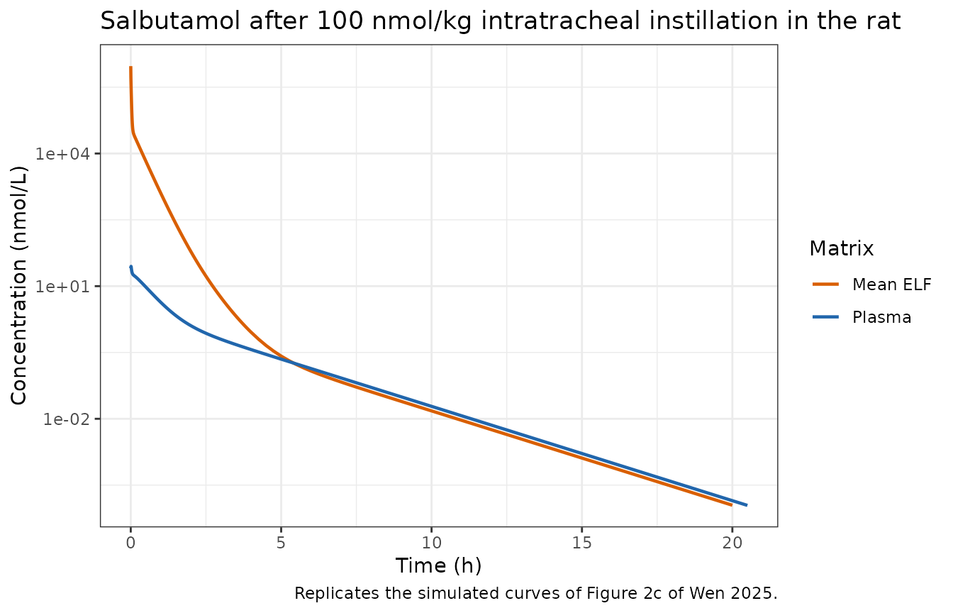
Replicate Appendix S2 Figure S9: regional and inter-tissue gradients
Wen 2025 reports two qualitative regional findings (section 3.3 and Appendix S2 Figure S9): the epithelium carries the highest drug concentration, followed by ELF and then subepithelium; and concentrations are higher in the central lung (generations 1-16) than in the peripheral lung (generations 17-24). Both are asserted below rather than only plotted.
long <- published |>
  dplyr::select(time, dplyr::matches("^(elf|epi|sub)_[0-9]{2}$")) |>
  tidyr::pivot_longer(-time, names_to = "state", values_to = "amount") |>
  tidyr::separate(state, into = c("layer", "gen"), sep = "_", convert = TRUE) |>
  dplyr::mutate(
    volume = dplyr::case_when(
      layer == "elf" ~ Velf[gen],
      layer == "epi" ~ Vepi[gen],
      TRUE           ~ rsub[gen] * (0.004126 * 0.35 - sum(Velf) - sum(Vepi))
    ),
    conc   = amount / volume,
    region = ifelse(gen <= 16, "Central (gen 1-16)", "Peripheral (gen 17-24)"),
    layer  = factor(layer, c("elf", "epi", "sub"),
                    c("ELF", "Epithelium", "Subepithelium"))
  )

layer_auc <- long |>
  dplyr::group_by(layer, gen) |>
  dplyr::summarise(auc = sum(diff(time) * (head(conc, -1) + tail(conc, -1)) / 2),
                   .groups = "drop") |>
  dplyr::group_by(layer) |>
  dplyr::summarise(`mean AUC (nmol*h/L)` = mean(auc), .groups = "drop")
knitr::kable(layer_auc, digits = 1,
caption = "Generation-averaged AUC by tissue layer (Appendix S2 Figure S9).")| layer | mean AUC (nmol*h/L) |
|---|---|
| ELF | 44046.6 |
| Epithelium | 141277.6 |
| Subepithelium | 1031.3 |
region_auc <- long |>
  dplyr::filter(layer == "ELF") |>
  dplyr::group_by(region, gen) |>
  dplyr::summarise(auc = sum(diff(time) * (head(conc, -1) + tail(conc, -1)) / 2),
                   .groups = "drop") |>
  dplyr::group_by(region) |>
  dplyr::summarise(`mean ELF AUC (nmol*h/L)` = mean(auc), .groups = "drop")
knitr::kable(region_auc, digits = 1,
caption = "Central vs peripheral lung ELF exposure (Wen 2025 section 3.3).")| region | mean ELF AUC (nmol*h/L) |
|---|---|
| Central (gen 1-16) | 59863.6 |
| Peripheral (gen 17-24) | 12412.6 |
# Published qualitative findings, asserted.
stopifnot(
  layer_auc$`mean AUC (nmol*h/L)`[layer_auc$layer == "Epithelium"] >
    layer_auc$`mean AUC (nmol*h/L)`[layer_auc$layer == "ELF"],
  layer_auc$`mean AUC (nmol*h/L)`[layer_auc$layer == "ELF"] >
    layer_auc$`mean AUC (nmol*h/L)`[layer_auc$layer == "Subepithelium"],
  region_auc$`mean ELF AUC (nmol*h/L)`[region_auc$region == "Central (gen 1-16)"] >
    region_auc$`mean ELF AUC (nmol*h/L)`[region_auc$region == "Peripheral (gen 17-24)"]
)

long |>
  dplyr::filter(time %in% c(0.5, 2, 6.25)) |>
  ggplot(aes(gen, conc, colour = layer)) +
  geom_line(linewidth = 0.7) +
  facet_wrap(~ paste0(time, " h"), scales = "free_y") +
  scale_y_log10() +
  labs(x = "Airway generation", y = "Concentration (nmol/L)", colour = "Layer",
       title = "Concentration by airway generation and tissue layer",
       caption = "Replicates Appendix S2 Figure S9 of Wen 2025.") +
  theme_bw()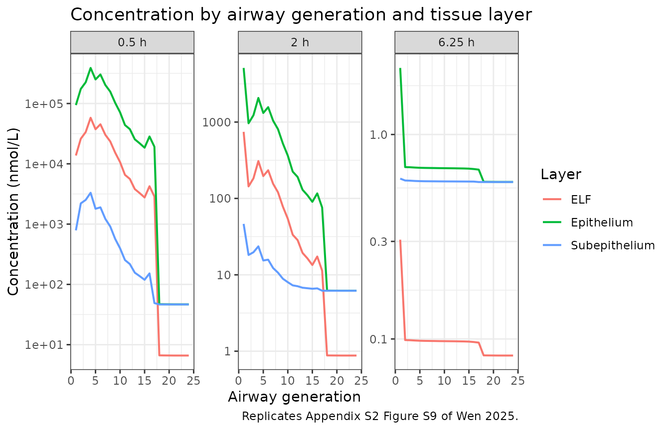
PKNCA validation
Wen 2025 reports no NCA table for the rat arm (Figure 2 is graphical,
and Table 3 covers the human translation only). The available
quantitative check is an exact structural identity: because
intratracheal instillation delivers the whole dose into the lung and the
only elimination pathway in the model is systemic clearance from the
central compartment, plasma AUC0-inf must equal
Dose / CL with the CL = 2.31 L/h of Table 1.
That identity holds per rat, at every body weight, and would break under
any error in the deposition fractions, the mass-transfer equations or
the blood-flow apportionment.
sim_nca <- sim |>
  dplyr::filter(!is.na(Cc)) |>
  dplyr::select(id, time, Cc, cohort)

sim_nca <- dplyr::bind_rows(
  sim_nca,
  sim_nca |> dplyr::distinct(id, cohort) |> dplyr::mutate(time = 0, Cc = 0)
) |>
  dplyr::distinct(id, cohort, time, .keep_all = TRUE) |>
  dplyr::arrange(id, cohort, time)

conc_obj <- PKNCA::PKNCAconc(sim_nca, Cc ~ time | cohort + id)

dose_df <- events |>
  dplyr::filter(evid == 1, cmt == "elf_01") |>
  dplyr::mutate(amt = amt) |>
  dplyr::select(id, time, amt, cohort)
dose_obj <- PKNCA::PKNCAdose(dose_df, amt ~ time | cohort + id)

# Linear-up/log-down keeps the trapezoidal error on the very steep early plasma
# rise small enough that the AUC identity below can be asserted tightly.
PKNCA::PKNCA.options(auc.method = "lin up/log down")

intervals <- data.frame(
  start = 0, end = Inf,
  cmax = TRUE, tmax = TRUE, aucinf.obs = TRUE, auclast = TRUE, half.life = TRUE
)

nca_res <- PKNCA::pk.nca(PKNCA::PKNCAdata(conc_obj, dose_obj, intervals = intervals))
Comparison against the analytic reference
cl_pub <- 2.31                                   # L/h, Wen 2025 Table 1
reference <- tibble::tibble(
  cohort     = c("300 g rat", "350 g rat", "400 g rat"),
  aucinf.obs = c(100 * 0.30, 100 * 0.35, 100 * 0.40) / cl_pub
)

cmp <- nlmixr2lib::ncaComparisonTable(
  simulated     = nca_res,
  reference     = reference,
  by            = "cohort",
  params        = "aucinf.obs",
  units         = c(aucinf.obs = "nmol*h/L"),
  tolerance_pct = 20
)
knitr::kable(cmp, caption = "Plasma AUC0-inf vs the analytic identity Dose / CL. * differs by >20%.")| NCA parameter | cohort | Reference | Simulated | % diff |
|---|---|---|---|---|
| AUC0-∞ (obs) (nmol*h/L) | 300 g rat | 13 | 13 | -0.1% |
| AUC0-∞ (obs) (nmol*h/L) | 350 g rat | 15.2 | 15.1 | -0.1% |
| AUC0-∞ (obs) (nmol*h/L) | 400 g rat | 17.3 | 17.3 | -0.1% |
# Strict form of the same test: the identity must hold to within 0.5%
# (the residual is trapezoidal error on the observation grid, not model error).
auc_sim <- as.data.frame(nca_res) |>
  dplyr::filter(PPTESTCD == "aucinf.obs") |>
  dplyr::arrange(cohort)
auc_ref <- reference |> dplyr::arrange(cohort)
stopifnot(all(abs(auc_sim$PPORRES / auc_ref$aucinf.obs - 1) < 0.005))
Lung-to-plasma exposure
The paper’s headline translational metric is the lung-to-plasma
AUClast ratio (Wen 2025 Table 3). Table 3 tabulates the
human values only; the rat value the model implies is reported here for
completeness.
trap <- function(t, y) sum(diff(t) * (head(y, -1) + tail(y, -1)) / 2)
ratio_tbl <- published |>
  dplyr::summarise(
    `Plasma AUClast (nmol*h/L)`   = trap(time, Cc),
    `Mean ELF AUClast (nmol*h/L)` = trap(time, Celf)
  ) |>
  dplyr::mutate(`Mean ELF : plasma ratio` = `Mean ELF AUClast (nmol*h/L)` /
                  `Plasma AUClast (nmol*h/L)`)
knitr::kable(ratio_tbl, digits = 1,
caption = "Rat mean-ELF to plasma AUC ratio over 0-24 h implied by the model.")| Plasma AUClast (nmol*h/L) | Mean ELF AUClast (nmol*h/L) | Mean ELF : plasma ratio |
|---|---|---|
| 15.1 | 20999.6 | 1387.4 |
Scope
Wen 2025 develops one framework and applies it in four combinations: two drugs (salbutamol, fluticasone propionate) in two species (rat, human). Only the rat salbutamol arm is packaged here. The other three are not reproducible from the available sources:
- Fluticasone propionate in the rat. Appendix S1 section 3.2 reports only the three regional MPPD deposition totals (head 0.9258, TB 0.0089, pulmonary 0.0158) after nose-only inhalation; the split of those totals across the individual generations is not reported. The particle-dissolution model of Appendix S1 Eq S18 additionally needs the aqueous diffusion coefficient, which Appendix S1 states is “estimated as a function of molecular weight in MoBi” but does not print.
-
Both drugs in the human. Appendix S1 section 6
states that human morphometry follows the Weibel lung model “with
detailed parameters presented in cited references” and does not
reproduce the table; the human ELF, epithelial and subepithelial
thicknesses are not reported anywhere; and the per-generation deposition
comes from running the Pellowe typical-path model rather than from a
printed table. The published MoBi project file named
PBPK for inhalation_humandoes not supply them - its spatial-structure building block still carries the rat parameterisation (maximum mucociliary clearance 0.019 cm/min = the rat’s 1.9 mm/min rather than the human 3.6 mm/min; total lung volume 0.001238 L rather than the human 0.53 L; alveolar surface 38.7 dm2 rather than 7000 dm2), because the human values were set at the simulation level and the project’sSIMULATIONStable was exported empty.
Filling any of those gaps would mean substituting values that are not in any available source, which the nlmixr2lib PBPK sourcing rule forbids.
Assumptions and deviations
- Dissolution and mucociliary clearance are inactive in this arm. The framework includes both, but Wen 2025 Table 1 reports no density, MMAD or GSD for salbutamol in the rat (the “predictive deposition parameters” row is blank), so the particle model of Appendix S1 Eqs S18-S19 cannot be parameterised and was not used: the intratracheal deposition of Eq S13 is a direct geometric rule, not an MPPD particle prediction. Salbutamol’s aqueous solubility of 14 100 mg/L (Table 1) corresponds to 58.9 mmol/L, roughly 60-fold above the peak mean ELF concentration the model predicts, so the instillate is fully dissolved and mucociliary clearance - which transports only undissolved particles (Wen 2025 section 2.2) - has nothing to move. The dose is therefore deposited directly into the ELF of each generation.
-
74.5%tracheobronchial deposition is not self-consistent. Appendix S1 section 3.2 states that Eq S13 gives “74.5% in TB region and 29.3% in alveolar region”, which sums to 103.8%. Evaluating Eq S13 over generations 1-24 gives 70.6% / 29.4%, matching the printed alveolar figure. The equation is used, per the standing policy of trusting a printed equation over conflicting prose; the geometry gate above asserts the 29.3% alveolar figure is reproduced. -
Eq S11 blood-flow weighting factor. Appendix S1 Eq
S11 gives
F_i = 0.19 + 2.8 * exp(-5.1 * D)withDin cm; the published MoBi project encodes0.19 + 2.8 * e^(-0.51 * D)withDin MoBi’s base length unit (dm), i.e. an exponent 100-fold smaller. The MoBi form makesF_ivary only between 2.94 and 2.99 across the whole tracheobronchial tree, which would make the weighting factor inert; Eq S11 as printed spans 0.69 to 2.96. Eq S11 is used. - Subepithelial region normalisers. The published MoBi project hard-codes the tracheobronchial and alveolar subepithelial volume sums as 0.0003676 L and 0.0007246 L. Those do not follow from the project’s own volume formulas applied to Table S2 (which give 0.000654 L and 0.000425 L), and the project file is otherwise a template whose drug-specific and simulation-level values were exported as zeros. The model therefore computes the regional sums from Eqs S5-S9 rather than adopting the hard-coded constants.
- Two Table S3 residence times are not reproducible. Generations 5 and 10 give 4.76 and 7.31 min from Eqs S15-S16 applied to Table S2, versus the tabulated 4.03 and 6.99 min. The other 14 agree exactly. Because mucociliary clearance is inactive in this arm the discrepancy does not affect any prediction here; it is recorded so that a future fluticasone-propionate extraction, where mucociliary clearance is active, resolves it first.
-
Kp,u,lunginitial value rounding. Eq 5 applied to Table 1 gives 4.66 / 0.71 = 6.56 for salbutamol, whereas Table 1 prints 6.50. This is the initial value only; the model uses the estimated 8.83 of section 3.2, so the rounding does not propagate. (Fluticasone propionate reproduces exactly: 3.41 / 0.016 = 213.1.) -
Equation numbering in Table 1. Table 1 cites
“Equation (6)” for
Kp,u,lungand “Equation (5)” forfu,ELF; in the article body those are Eqs 5 and 4 respectively. The arithmetic identifies the intended equations unambiguously. -
No random effects and no residual error. Wen 2025
reports neither, so
propSdandpropSd_Celfare fixed placeholders (0.10) that exist only so the two observed matrices have declared endpoints. Do not read them as published precision estimates. -
Body weight. Airway number, length and diameter are
the fixed Yeh lung-cast morphometry of a 330 g rat and are not
scaled with
WT; only lung volume and cardiac output scale (Appendix S1 section 3.1). The published salbutamol arm used 350 g rats. - Observed data are not redistributed. The rat plasma and BAL ELF points of Figure 2 were digitised by Wen 2025 from Boger and Friden (2019) and are not included in this package, so the figure chunk shows the simulated curves only.