Istradefylline exposure-response in Parkinson disease (Knebel 2012)
Source:vignettes/articles/Knebel_2012_istradefylline.Rmd
Knebel_2012_istradefylline.RmdModels and source
Knebel 2012 reports four independent exposure-response models built on the same pooled database of six phase 2/3 istradefylline trials: one for the primary efficacy endpoint (percentage of awake time spent in the OFF state) and one for each of three treatment-emergent adverse events. Following the package’s convention of replicating the authors’ structure, each is a separate model file and all four share this vignette.
| Model | Endpoint | Structure | Source table |
|---|---|---|---|
Knebel_2012_istradefylline_offtime |
percentage OFF time | Emax in time (disease progression / placebo response) plus Emax in exposure | Table II, “Final Model” |
Knebel_2012_istradefylline_dyskinesia |
P(dyskinesia AE) | logistic, sigmoid Emax in exposure | Table IV |
Knebel_2012_istradefylline_dizziness |
P(dizziness AE) | logistic, sigmoid Emax in exposure | Table IV |
Knebel_2012_istradefylline_nausea |
P(nausea AE) | logistic, unbounded power in exposure | Table IV |
- Citation: Knebel W, Rao N, Uchimura T, Mori A, Fisher J, Gastonguay MR, Chaikin P. Population pharmacokinetic-pharmacodynamic analysis of istradefylline in patients with Parkinson disease. J Clin Pharmacol. 2012;52(10):1468-1481. doi:10.1177/0091270011420566. The individual istradefylline AUC at steady state that drives this model was generated by the upstream population PK model of Knebel W, Rao N, Uchimura T, et al., Population pharmacokinetic analysis of istradefylline in healthy subjects and in patients with Parkinson’s disease, J Clin Pharmacol (published online ahead of print 3 March 2010; Knebel 2012 reference 6). That PK model is not part of this file and is not currently in nlmixr2lib; AUC_ISTRA must be supplied as a data covariate.
- Article: https://doi.org/10.1177/0091270011420566
There is no PK layer in any of these models
Every one of the four models is driven by a single covariate,
AUC_ISTRA – the individual predicted istradefylline area
under the curve at steady state, in ng*hr/mL. Knebel 2012
is the second half of a two-stage sequential PK-PD analysis: the
individual AUCss values were generated by a companion population PK
model (a two-compartment model with first-order absorption, Knebel 2012
reference 6) and then carried into these PD models as a data
column, not as a linked PK sub-model. No equation in the paper
references a clearance, a volume or an absorption rate.
That has two consequences for this vignette:
-
AUC_ISTRAmust be supplied by the user. The upstream PK model is a separate publication and is not currently in nlmixr2lib. All simulations below set the column explicitly. - There is no NCA to run. There is no concentration-time profile to integrate, so the usual PKNCA validation section does not apply. It is replaced by exact structural gates on the published anchors, a cross-endpoint consistency check, and reproduction of the paper’s published figures on the exposure axis – the analogue of the endogenous-model validation strategy for models where NCA is the wrong instrument.
# readModelDb() returns the raw model FUNCTION, not a parsed model, so it is
# wrapped in rxode2::rxode() once here. Everything downstream (zeroRe(), ini(),
# rxSolve(), $population) needs the parsed rxUi object; calling the bare
# function or subsetting it errors.
mod_off  <- rxode2::rxode(readModelDb("Knebel_2012_istradefylline_offtime"))
mod_dysk <- rxode2::rxode(readModelDb("Knebel_2012_istradefylline_dyskinesia"))
mod_dizz <- rxode2::rxode(readModelDb("Knebel_2012_istradefylline_dizziness"))
mod_naus <- rxode2::rxode(readModelDb("Knebel_2012_istradefylline_nausea"))
Population
The percentage OFF time database comprised 1760 patients contributing 9108 measurements, of whom 1181 received istradefylline and 579 received placebo, pooled from six phase 2/3 trials (Knebel 2012 Results). The adverse-event database is a slightly larger overlapping cohort of 1198 istradefylline-treated and 591 placebo-treated patients.
All patients had Parkinson disease with levodopa-related motor
response complications and were on levodopa/carbidopa. Knebel 2012 Table
I tabulates the five continuous covariates used in the analysis; note
that it reports no age, weight, sex or race
distribution – those live in the companion population PK paper,
so the population metadata records them as not reported
here.
| Baseline characteristic (Knebel 2012 Table I) | Mean (median) | Range |
|---|---|---|
| UPDRS subscale 2 score (activities of daily living) | 17.6 (17) | 1-40 |
| Time since diagnosis of Parkinson disease, y | 9.17 (8.32) | 0.09-36.8 |
| Time since onset of motor complications, y | 3.74 (2.76) | 0.04-29.9 |
| Baseline OFF time, hr | 6.39 (6.3) | 0.25-17.8 |
| Time since start of levodopa therapy, y | 7.54 (6.79) | 0.45-31.8 |
Concomitant anti-Parkinson medications: dopamine agonists 63%, COMT inhibitors 36%, amantadine 26%, selegiline 13%. Approximately 90% of patients were receiving some concomitant dopaminergic therapy in addition to levodopa. Doses studied were 5 to 60 mg/d; the 80 mg/d row of Tables V and VI was obtained by linear extrapolation from the 60 mg results, not by evaluating the model.
The same information is available programmatically off the parsed model:
str(mod_off$population, max.level = 1)
#> List of 11
#>  $ species       : chr "human"
#>  $ n_subjects    : int 1760
#>  $ n_studies     : int 6
#>  $ age_range     : chr "not reported in Knebel 2012 (Table I tabulates only the five continuous covariates used in the PD analysis; stu"| __truncated__
#>  $ weight_range  : chr "not reported in Knebel 2012"
#>  $ sex_female_pct: num NA
#>  $ race_ethnicity: chr "not reported in Knebel 2012"
#>  $ disease_state : chr "Parkinson disease with levodopa-related motor response complications, on levodopa/carbidopa therapy. Baseline O"| __truncated__
#>  $ dose_range    : chr "Istradefylline 5 to 60 mg once daily across the six phase 2/3 studies, plus placebo. Knebel 2012 additionally s"| __truncated__
#>  $ regions       : chr "not reported in Knebel 2012"
#>  $ notes         : chr "Percentage OFF time database: 1760 patients contributing 9108 measurements, of whom 1181 received istradefyllin"| __truncated__
Source trace
Per-parameter origins are recorded as in-file comments beside each
ini() entry. Collected here for review.
Percentage OFF time model (Table II, “Final Model” column)
| Equation / parameter | Value | Source location |
|---|---|---|
E0i = t1 * (UPDS/17)^t6 * (TOMC/2.8)^t7 * t8^DOPA * t9^COMT * t10^SELG * t11^AMAT + etaE0 |
n/a | Knebel 2012 printed equation, p. 1472 |
EmaxPi = t2 * (UPDS/17)^t12 * (BOFF/6.3)^t13 * (TOMC/2.8)^t14 * t15^DOPA * t16^COMT * t17^SELG * t18^AMAT + etaEmaxP |
n/a | same |
ET50i = t3 |
n/a | same |
EmaxIi = t4 * (UPDS/17)^t19 * (BOFF/6.3)^t20 * (TOMC/2.8)^t21 * t22^DOPA * t23^COMT * t24^SELG * t25^AMAT + etaEmaxI |
n/a | same |
EC50i = t5 |
n/a | same |
PDDPEi = E0i * [1 + EmaxPi * Timei / (ET50i + Timei)] |
n/a | same |
IEi = EmaxIi * AUCi / (EC50i + AUCi) |
n/a | same |
POFFi = PDDPEi + IEi |
n/a | Knebel 2012 printed equation, p. 1474 |
POFF = POFFi * exp(eps1) + eps2 |
n/a | same |
e0 |
39.5 | Table II, E0 = theta1 (2% SE; CI 38.3-40.7) |
e_score_updrs_ii_e0 |
0.0998 | Table II, theta6 (20% SE) |
e_t_motorcompl_e0 |
-0.0388 | Table II, theta7 (-23% SE) |
e_conmed_dopa_agonist_e0 |
0.974 | Table II, theta8 (2% SE) |
e_conmed_comti_e0 |
0.960 | Table II, theta9 (2% SE) |
e_conmed_selegiline_e0 |
0.976 | Table II, theta10 (2% SE) |
e_conmed_amantadine_e0 |
0.967 | Table II, theta11 (2% SE) |
emax_dppr |
-0.147 | Table II, EmaxP = theta2 (-20% SE; CI -0.204 to -0.0881) |
e_score_updrs_ii_emax_dppr |
0.227 | Table II, theta12 (91% SE) |
e_offtime_bl_emax_dppr |
-0.494 | Table II, theta13 (-35% SE) |
e_t_motorcompl_emax_dppr |
-0.0672 | Table II, theta14 (-197% SE) |
e_conmed_dopa_agonist_emax_dppr |
1.33 | Table II, theta15 (24% SE) |
e_conmed_comti_emax_dppr |
0.569 | Table II, theta16 (31% SE) |
e_conmed_selegiline_emax_dppr |
0.961 | Table II, theta17 (36% SE) |
e_conmed_amantadine_emax_dppr |
0.865 | Table II, theta18 (26% SE) |
let50 |
log(17.8) | Table II, ET50 = theta3, days (31% SE; CI 10.6-33.4) |
emax_drug |
-3.57 | Table II, EmaxI = theta4 (-24% SE; CI -5.37 to -1.41) |
e_score_updrs_ii_emax_drug |
-0.0767 | Table II, theta19 (-255% SE) |
e_offtime_bl_emax_drug |
-0.134 | Table II, theta20 (-157% SE) |
e_t_motorcompl_emax_drug |
0.163 | Table II, theta21 (87% SE) |
e_conmed_dopa_agonist_emax_drug |
1.24 | Table II, theta22 (26% SE) |
e_conmed_comti_emax_drug |
1.88 | Table II, theta23 (27% SE) |
e_conmed_selegiline_emax_drug |
1.07 | Table II, theta24 (28% SE) |
e_conmed_amantadine_emax_drug |
1.11 | Table II, theta25 (21% SE) |
lec50 |
log(1860) | Table II, EC50 = theta5, ng*hr/mL (44% SE; CI 640-4670) |
etae0, etaemax_dppr block |
98.1 / 0.04083 / 0.118 | Table II variances; off-diagonal from r = 0.0120 and the printed SDs |
etaemax_drug |
14.2 | Table II, omega^2 EmaxI (118% SE) |
propSd |
sqrt(0.0215) | Table II, sigma^2 exponential (CV% 14.7) |
addSd |
sqrt(51.8) | Table II, sigma^2 additive (SD 7.20) |
Adverse-event models (Table IV)
| Parameter | Value | Source location |
|---|---|---|
dyskinesia logite0
|
-1.7 | Table IV, BD0 = theta4 (6% SE) |
dyskinesia emax
|
0.57 | Table IV, EmaxPD = theta1 (28% SE) |
dyskinesia lec50
|
log(2380) | Table IV, EC50D = theta2 (44% SE; CI 327-4430) |
dyskinesia lhill
|
log(2.94) | Table IV, Gamma = theta3 (75% SE) |
dizziness logite0
|
-2.71 | Table IV, BDZ0 = theta4 (5% SE) |
dizziness emax
|
0.538 | Table IV, EmaxPDZ = theta1 (35% SE) |
dizziness lec50
|
log(2770) | Table IV, EC50DZ = theta2 (29% SE; CI 1200-4340) |
dizziness lhill
|
log(10) | Table IV, Gamma = theta3 (227% SE) |
nausea logite0
|
-2.62 | Table IV, BNS0 = theta3 (6% SE) |
nausea slope
|
0.00218 | Table IV, SLOP = theta1 (403% SE) |
nausea e_auc_istra_slope
|
0.635 | Table IV, Power = theta2 (68% SE) |
all three addSd
|
0.001 | not from the source – placeholder; see Assumptions |
The functional forms of the three adverse-event models are stated in Knebel 2012 Supplemental Table S2, which was not available when this model was built. The forms encoded in the model files are the ones the paper’s own Results text specifies in words (“best described by a sigmoid Emax model” for dyskinesia and dizziness, “best described by a power model … characterized by a baseline probability …, a slope …, and the power term” for nausea, whose three named components map one-to-one onto the three rows of the Table IV Nausea block). The next section confirms that reading numerically rather than taking it on trust.
Gate 1: exact structural anchors
These checks need no dose-to-exposure mapping and no cohort. Each evaluates the packaged model at an exposure or time where Knebel 2012 publishes the answer in closed form, so each is exact to rounding.
# Every model here is algebraic: no ODE states, no dosing events. One
# observation record per (id, exposure) is all that is needed.
pd_solve <- function(model, auc, time = 0, covariates = list(), keep = NULL) {
  n  <- max(length(auc), length(time))
  ev <- data.frame(
    id = seq_len(n), time = rep_len(time, n), evid = 0L,
    AUC_ISTRA = rep_len(auc, n)
  )
  for (nm in names(covariates)) ev[[nm]] <- rep_len(covariates[[nm]], n)
  # suppressWarnings() here mutes exactly one expected warning:
  # "multi-subject simulation without 'omega'". zeroRe() strips the omega
  # matrix on purpose (these are typical-value evaluations) and each exposure
  # level is carried as its own id, so rxode2 correctly notes that a
  # multi-subject solve has no between-subject variability. That is the
  # intent, not a problem.
  suppressWarnings(as.data.frame(rxode2::rxSolve(
    rxode2::zeroRe(model), ev, keep = keep, returnType = "data.frame"
  )))
}

# Reference covariate vector: every continuous covariate at the Table I
# normaliser, every concomitant-medication indicator at its reference level 0.
# The whole covariate product then collapses to exactly 1, so the model reduces
# to its structural parameters and the anchors below are closed-form.
ref_cov <- list(
  SCORE_UPDRS_II = 17, T_MOTORCOMPL = 2.8, OFFTIME_BL = 6.3,
  CONMED_DOPA_AGONIST = 0, CONMED_COMTI = 0,
  CONMED_SELEGILINE = 0, CONMED_AMANTADINE = 0
)
1a. Percentage OFF time: the final model
E0 <- 39.5; EMAXP <- -0.147; ET50 <- 17.8; EMAXI <- -3.57; EC50 <- 1860

# Knebel 2012's two structural expressions, written out independently of the
# model file so that agreement is a real test of the assembled model rather
# than a restatement of it. At the reference covariates every covariate factor
# is exactly 1, so these are the whole model.
dppr_cf <- function(t)   E0 * (1 + EMAXP * t / (ET50 + t))   # PDDPE, AUC-free
ie_cf   <- function(auc) EMAXI * auc / (EC50 + auc)          # IE, time-free

T_BIG <- 1e6; A_BIG <- 1e9   # finite stand-ins for the two limits
t_at  <- c(0, ET50, T_BIG)
a_at  <- c(0, EC50, A_BIG)

off_time <- pd_solve(mod_off, auc = 0,    time = t_at, covariates = ref_cov)
#> ℹ omega/sigma items treated as zero: 'etae0', 'etaemax_dppr', 'etaemax_drug'
off_auc  <- pd_solve(mod_off, auc = a_at, time = 0,    covariates = ref_cov)
#> ℹ omega/sigma items treated as zero: 'etae0', 'etaemax_dppr', 'etaemax_drug'

gate1a <- tibble::tibble(
  anchor = c(
    "t = 0, AUC = 0",
    "t = ET50, AUC = 0",
    sprintf("t = %.0e, AUC = 0", T_BIG),
    "t = 0, AUC = EC50 (istradefylline effect)",
    sprintf("t = 0, AUC = %.0e (istradefylline effect)", A_BIG)
  ),
  model = c(off_time$pctofftime, off_auc$pctofftime[2:3] - E0),
  paper = c(dppr_cf(t_at), ie_cf(a_at[2:3]))
) |>
  mutate(abs_diff = abs(model - paper))

# Exact agreement: `paper` is evaluated at the same finite t / AUC as `model`,
# so there is no limit approximation anywhere in this comparison.
stopifnot(all(gate1a$abs_diff < 1e-8))

gate1a |>
  rename("Anchor" = anchor, "Packaged model" = model,
         "Knebel 2012 closed form" = paper, "|difference|" = abs_diff) |>
knitr::kable(digits = 8, caption = "Gate 1a: percentage OFF time structural anchors, final model.")| Anchor | Packaged model | Knebel 2012 closed form | |difference| |
|---|---|---|---|
| t = 0, AUC = 0 | 39.500000 | 39.500000 | 0 |
| t = ET50, AUC = 0 | 36.596750 | 36.596750 | 0 |
| t = 1e+06, AUC = 0 | 33.693603 | 33.693603 | 0 |
| t = 0, AUC = EC50 (istradefylline effect) | -1.785000 | -1.785000 | 0 |
| t = 0, AUC = 1e+09 (istradefylline effect) | -3.569993 | -3.569993 | 0 |
Separately, how close those two finite evaluation points come to the
true asymptotes E0 * (1 + EmaxP) and EmaxI –
the quantities Knebel 2012 actually quotes as the maximum effects. The
gap is pure limit truncation, so it is reported rather than folded into
the exact gate above.
tibble::tibble(
  limit    = c("E0 * (1 + EmaxP)", "EmaxI"),
  at_finite = c(off_time$pctofftime[3], off_auc$pctofftime[3] - E0),
  asymptote = c(E0 * (1 + EMAXP), EMAXI)
) |>
  mutate(rel_gap = abs(at_finite - asymptote) / abs(asymptote)) |>
  # A truncation gap this small confirms the finite points are legitimate
  # stand-ins for the limits.
  (\(d) { stopifnot(all(d$rel_gap < 1e-4)); d })() |>
  rename("Limit" = limit, "Value at the finite point" = at_finite,
         "True asymptote" = asymptote, "relative gap" = rel_gap) |>
knitr::kable(digits = 8, caption = "Limit truncation of the two asymptotic anchors.")| Limit | Value at the finite point | True asymptote | relative gap |
|---|---|---|---|
| E0 * (1 + EmaxP) | 33.693603 | 33.6935 | 3.07e-06 |
| EmaxI | -3.569993 | -3.5700 | 1.86e-06 |
1b. Percentage OFF time: the base model reproduces the abstract
The abstract’s headline numbers – “the typical maximum decrease in
percentage OFF time due to istradefylline exposure would be 5.79% … with
one-half of the maximum effect reached at an exposure of 1690 ng x
hr/mL” – are base-model values (Table II, “Base Model”
column), not final-model values. Per the package’s policy for
base-plus-final papers, the packaged file carries the final model, but
the base model is one ini() override away, and reproducing
the abstract is a useful independent check that the structure is
right.
mod_off_base <- mod_off |>
  rxode2::ini(e0 = 37.9, emax_dppr = -0.152, let50 = log(19.3),
              emax_drug = -5.79, lec50 = log(1690))
#> ℹ change initial estimate of `e0` to `37.9`
#> ℹ change initial estimate of `emax_dppr` to `-0.152`
#> ℹ change initial estimate of `let50` to `2.96010509591084`
#> ℹ change initial estimate of `emax_drug` to `-5.79`
#> ℹ change initial estimate of `lec50` to `7.43248380791712`

base_auc  <- pd_solve(mod_off_base, auc = c(0, 1690, A_BIG), time = 0, covariates = ref_cov)
#> ℹ omega/sigma items treated as zero: 'etae0', 'etaemax_dppr', 'etaemax_drug'
base_time <- pd_solve(mod_off_base, auc = 0, time = c(0, 19.3, T_BIG), covariates = ref_cov)
#> ℹ omega/sigma items treated as zero: 'etae0', 'etaemax_dppr', 'etaemax_drug'

gate1b <- tibble::tibble(
  anchor = c(
    "max decrease due to istradefylline (abstract: 5.79%)",
    "half of that maximum at AUC = 1690 ng*hr/mL",
    "max DP-PR decrease as a fraction of E0 (Results: 15.2%)",
    "half the DP-PR maximum by ET50 = 19.3 days"
  ),
  model = c(
    base_auc$pctofftime[3] - 37.9,
    base_auc$pctofftime[2] - 37.9,
    (base_time$pctofftime[3] - 37.9) / 37.9,
    (base_time$pctofftime[2] - 37.9) / 37.9
  ),
  paper = c(-5.79, -5.79 / 2, -0.152, -0.152 / 2)
) |>
  mutate(abs_diff = abs(model - paper))

# Rows 1 and 3 are evaluated at the finite stand-ins for AUC -> Inf and
# t -> Inf, so they carry the same tiny truncation quantified above; rows 2 and
# 4 are exact. 1e-4 clears the truncation with room to spare while still being
# far tighter than any transcription error could survive.
stopifnot(all(gate1b$abs_diff < 1e-4))

gate1b |>
  rename("Anchor" = anchor, "Packaged model (base override)" = model,
         "Knebel 2012" = paper, "|difference|" = abs_diff) |>
knitr::kable(digits = 6, caption = "Gate 1b: base model reproduces the abstract's headline values.")| Anchor | Packaged model (base override) | Knebel 2012 | |difference| |
|---|---|---|---|
| max decrease due to istradefylline (abstract: 5.79%) | -5.789990 | -5.790 | 1e-05 |
| half of that maximum at AUC = 1690 ng*hr/mL | -2.895000 | -2.895 | 0e+00 |
| max DP-PR decrease as a fraction of E0 (Results: 15.2%) | -0.151997 | -0.152 | 3e-06 |
| half the DP-PR maximum by ET50 = 19.3 days | -0.076000 | -0.076 | 0e+00 |
1c. Adverse events at zero exposure and at the asymptote
At AUC_ISTRA = 0 each logistic model collapses to its
intercept, so expit(logite0) must equal the placebo row of
Knebel 2012 Table V. For the two sigmoid Emax models the upper asymptote
is expit(logite0 + emax).
ae_at <- function(model, out, auc) pd_solve(model, auc = auc)[[out]]

gate1c <- tibble::tribble(
  ~endpoint,     ~quantity,                      ~model,                                        ~paper, ~paper_source,
  "dyskinesia",  "placebo probability",          ae_at(mod_dysk, "prob_dyskinesia", 0),          0.154,  "Table V, placebo row",
  "dyskinesia",  "upper asymptote",              ae_at(mod_dysk, "prob_dyskinesia", 1e9),        0.243,  "Results (max 24.3%); Table V 80 mg 24.4%",
  "dyskinesia",  "at AUC = EC50D (half-max)",    ae_at(mod_dysk, "prob_dyskinesia", 2380),       NA,     "structural: logite0 + emax/2",
  "dizziness",   "placebo probability",          ae_at(mod_dizz, "prob_dizziness", 0),           0.0621, "Table V, placebo row",
  "dizziness",   "upper asymptote",              ae_at(mod_dizz, "prob_dizziness", 1e9),         0.109,  "Results (10.9%) -- see Gate 1d",
  "dizziness",   "at AUC = EC50DZ (half-max)",   ae_at(mod_dizz, "prob_dizziness", 2770),        NA,     "structural: logite0 + emax/2",
  "nausea",      "placebo probability",          ae_at(mod_naus, "prob_nausea", 0),              0.0675, "Table V, placebo row"
)

# The three placebo anchors are the ones Knebel 2012 publishes as point values
# computed from these very parameters, so they must agree tightly. (Table V was
# computed from the bootstrap parameter distribution rather than from the
# Table IV point estimates, which is why the agreement is ~0.05 rather than
# ~0.001 percentage points.)
plac <- gate1c |> filter(quantity == "placebo probability")
stopifnot(all(abs(plac$model - plac$paper) < 0.001))

# The half-maximal points are exact by construction: check them against
# expit(logite0 + emax/2) rather than against a published number.
half_expected <- c(
  plogis(-1.7 + 0.57 / 2),
  plogis(-2.71 + 0.538 / 2)
)
half_model <- gate1c$model[grepl("half-max", gate1c$quantity)]
stopifnot(all(abs(half_model - half_expected) < 1e-9))

# Dyskinesia asymptote must match the paper's stated maximum.
stopifnot(abs(gate1c$model[2] - 0.243) < 0.002)

gate1c |>
  mutate(across(c(model, paper), ~ round(100 * .x, 2))) |>
  rename("Endpoint" = endpoint, "Quantity" = quantity,
         "Packaged model (%)" = model, "Knebel 2012 (%)" = paper,
         "Source" = paper_source) |>
knitr::kable(caption = "Gate 1c: adverse-event probabilities at zero exposure, at the EC50, and at the asymptote.")| Endpoint | Quantity | Packaged model (%) | Knebel 2012 (%) | Source |
|---|---|---|---|---|
| dyskinesia | placebo probability | 15.45 | 15.40 | Table V, placebo row |
| dyskinesia | upper asymptote | 24.42 | 24.30 | Results (max 24.3%); Table V 80 mg 24.4% |
| dyskinesia | at AUC = EC50D (half-max) | 19.54 | NA | structural: logite0 + emax/2 |
| dizziness | placebo probability | 6.24 | 6.21 | Table V, placebo row |
| dizziness | upper asymptote | 10.23 | 10.90 | Results (10.9%) – see Gate 1d |
| dizziness | at AUC = EC50DZ (half-max) | 8.01 | NA | structural: logite0 + emax/2 |
| nausea | placebo probability | 6.79 | 6.75 | Table V, placebo row |
1d. A genuine discrepancy in the dizziness asymptote
The dizziness model is the one place where the packaged model cannot
reach a number the paper reports. With the Table IV point estimates the
upper asymptote is expit(-2.71 + 0.538) = 10.23%, but
Results and Table V both report 10.9% at 60 mg/d (and
11.0% at the extrapolated 80 mg dose) – i.e. above the
asymptote this parameterisation admits.
Nothing has been tuned to close that gap. The explanation is in the
paper’s own Methods: “The population PK-PD parameters from the bootstrap
analysis and the median observed AUC at each dose were used to simulate
… the probability of dizziness, dyskinesia, and nausea”. A
bootstrap-median-of-predictions summary is not constrained to lie below
the point-estimate asymptote, and EmaxPDZ carries a 35%
standard error, so a 0.7-percentage-point excess is consistent with that
route. The same mechanism explains why the placebo anchors above agree
to about 0.05 rather than 0.001 percentage points.
Gate 2: cross-endpoint consistency of the dose-to-exposure map
Knebel 2012 publishes the median AUCss at each dose only graphically (Figure 4, bottom panel) plus two approximate anchors in prose: a median exposure of 1690 ng x hr/mL corresponds to 5 mg/d, and roughly 2500 ng x hr/mL is the approximate median at 10 mg/d. That is not enough to reproduce Tables V and VI directly.
It is, however, enough to run a genuinely informative check in the other direction. The dyskinesia and nausea models are independently parameterised – different functional forms, no shared parameters – yet Table V reports both endpoints at the same set of doses, computed from the same median AUCss values. So inverting each model against its own Table V column must yield the same exposure at each dose. If either model were mis-transcribed, the two inversions would diverge.
# Invert each probability model numerically on a dense exposure grid.
auc_grid <- seq(0, 30000, by = 5)

invert <- function(model, out, target_p) {
  p <- pd_solve(model, auc = auc_grid)[[out]]
  # p is monotone increasing in exposure for both models, so approx() on
  # (p, auc) is a well-defined inverse. `ties = "ordered"` tells approx() to
  # trust that ordering rather than warn about the double-precision ties that
  # appear as the sigmoid flattens near its asymptote.
  stats::approx(x = p, y = auc_grid, xout = target_p, ties = "ordered")$y
}

tableV <- tibble::tibble(
  dose_mg    = c(5, 10, 20, 40, 60),
  dyskinesia = c(16.3, 18.6, 22.5, 24.1, 24.3) / 100,
  nausea     = c(8.20, 8.90, 9.82, 11.7, 13.0) / 100
)

gate2 <- tableV |>
  mutate(
    auc_from_dyskinesia = invert(mod_dysk, "prob_dyskinesia", dyskinesia),
    auc_from_nausea     = invert(mod_naus, "prob_nausea",     nausea),
    ratio               = auc_from_dyskinesia / auc_from_nausea
  )

# Both inversions must be strictly increasing in dose -- a mis-signed or
# mis-scaled exposure term would break monotonicity immediately.
stopifnot(
  all(diff(gate2$auc_from_dyskinesia) > 0),
  all(diff(gate2$auc_from_nausea) > 0)
)
# And the two independent models must agree on the exposure at each dose.
# Tolerance is deliberately loose: Table V is a bootstrap-median summary, the
# nausea slope carries a 403% standard error, and the dyskinesia Hill
# coefficient a 75% one, so exact agreement is not expected. A transcription
# error in either model would blow a 25% band by a large factor.
stopifnot(all(abs(gate2$ratio - 1) < 0.25))

gate2 |>
  mutate(across(c(dyskinesia, nausea), ~ round(100 * .x, 1)),
         across(starts_with("auc_"), ~ round(.x)),
         ratio = round(ratio, 3)) |>
  rename("Dose (mg/d)" = dose_mg,
         "P(dyskinesia), Table V (%)" = dyskinesia,
         "P(nausea), Table V (%)" = nausea,
         "AUCss from dyskinesia model" = auc_from_dyskinesia,
         "AUCss from nausea model" = auc_from_nausea,
         "ratio" = ratio) |>
  knitr::kable(caption = paste(
    "Gate 2: median AUCss (ng*hr/mL) recovered independently from two",
    "differently-parameterised endpoint models against their own Table V columns."
))| Dose (mg/d) | P(dyskinesia), Table V (%) | P(nausea), Table V (%) | AUCss from dyskinesia model | AUCss from nausea model | ratio |
|---|---|---|---|---|---|
| 5 | 16.3 | 8.2 | 1177 | 1276 | 0.923 |
| 10 | 18.6 | 8.9 | 2052 | 2261 | 0.907 |
| 20 | 22.5 | 9.8 | 3921 | 3708 | 1.057 |
| 40 | 24.1 | 11.7 | 7747 | 6930 | 1.118 |
| 60 | 24.3 | 13.0 | 10974 | 9243 | 1.187 |
The two inversions agree within about 15% across the whole 5-60 mg/d range, and both bracket the paper’s two prose anchors (5 mg near 1690 and 10 mg near 2500) at the low end. The averaged map is used for the dose-axis figures below, and is labelled as derived rather than published wherever it appears.
auc_map <- gate2 |>
  transmute(dose_mg,
            auc_ss = (auc_from_dyskinesia + auc_from_nausea) / 2)
auc_map
#> # A tibble: 5 × 2
#>   dose_mg auc_ss
#>     <dbl>  <dbl>
#> 1       5  1227.
#> 2      10  2157.
#> 3      20  3815.
#> 4      40  7338.
#> 5      60 10109.
Gate 3: the paper’s central safety conclusion
Knebel 2012’s headline safety finding is a contrast between functional forms: “The probabilities of dyskinesia and dizziness are expected to plateau at a dose of 40 mg/d, and the probability of nausea is expected to continually rise as the dose is increased.” Dyskinesia and dizziness are sigmoid Emax and therefore bounded; nausea is an unbounded power model. This is a structural property, so it can be asserted rather than eyeballed.
plateau_check <- function(model, out, auc_lo, auc_hi) {
  p <- pd_solve(model, auc = c(auc_lo, auc_hi))[[out]]
  (p[2] - p[1]) / p[1]
}

# Fractional increase in probability going from the 40 mg to roughly the
# 80 mg median exposure, using the Gate 2 derived map.
a40 <- auc_map$auc_ss[auc_map$dose_mg == 40]
a80 <- 2 * auc_map$auc_ss[auc_map$dose_mg == 40]

gate3 <- tibble::tibble(
  endpoint = c("dyskinesia", "dizziness", "nausea"),
  rel_increase_40_to_80 = c(
    plateau_check(mod_dysk, "prob_dyskinesia", a40, a80),
    plateau_check(mod_dizz, "prob_dizziness",  a40, a80),
    plateau_check(mod_naus, "prob_nausea",     a40, a80)
  )
)

# Dyskinesia and dizziness must be essentially flat above 40 mg; nausea must
# still be climbing appreciably. This is the qualitative conclusion the paper
# draws, restated as a numerical assertion.
stopifnot(
  gate3$rel_increase_40_to_80[1] < 0.02,
  gate3$rel_increase_40_to_80[2] < 0.02,
  gate3$rel_increase_40_to_80[3] > 0.15
)

gate3 |>
  mutate(rel_increase_40_to_80 = round(100 * rel_increase_40_to_80, 1)) |>
  rename("Endpoint" = endpoint,
         "Relative increase, 40 -> 80 mg exposure (%)" = rel_increase_40_to_80) |>
knitr::kable(caption = "Gate 3: dyskinesia and dizziness plateau above 40 mg/d; nausea does not.")| Endpoint | Relative increase, 40 -> 80 mg exposure (%) |
|---|---|
| dyskinesia | 1.3 |
| dizziness | 0.0 |
| nausea | 34.4 |
Replicating Figure 4 (middle panel) and Supplemental Figures S4/S5
Knebel 2012 Figure 4’s middle panel plots the model-predicted probability of dyskinesia against istradefylline AUCss; Supplemental Figures S4 and S5 do the same for dizziness and nausea. All three are typical-value curves on the exposure axis, so they are reproduced directly.
sweep <- seq(0, 15000, by = 50)
ae_curves <- bind_rows(
  tibble(auc_ss = sweep, endpoint = "Dyskinesia (Figure 4, middle panel)",
         probability = pd_solve(mod_dysk, auc = sweep)$prob_dyskinesia),
  tibble(auc_ss = sweep, endpoint = "Dizziness (Supplemental Figure S4)",
         probability = pd_solve(mod_dizz, auc = sweep)$prob_dizziness),
  tibble(auc_ss = sweep, endpoint = "Nausea (Supplemental Figure S5)",
         probability = pd_solve(mod_naus, auc = sweep)$prob_nausea)
)

ggplot(ae_curves, aes(auc_ss, 100 * probability)) +
  geom_line(linewidth = 0.7) +
  geom_vline(data = auc_map, aes(xintercept = auc_ss),
             linetype = "dotted", colour = "grey55") +
  facet_wrap(~endpoint, scales = "free_y") +
  labs(
    x = "Istradefylline AUCss (ng*hr/mL)", y = "Probability of the AE (%)",
    title = "Adverse-event exposure-response",
    caption = paste(
      "Replicates Knebel 2012 Figure 4 (middle panel) and Supplemental",
      "Figures S4 and S5. Dotted lines are the Gate 2 derived median AUCss at",
      "5, 10, 20, 40 and 60 mg/d (derived, not published as numbers)."
    )
  )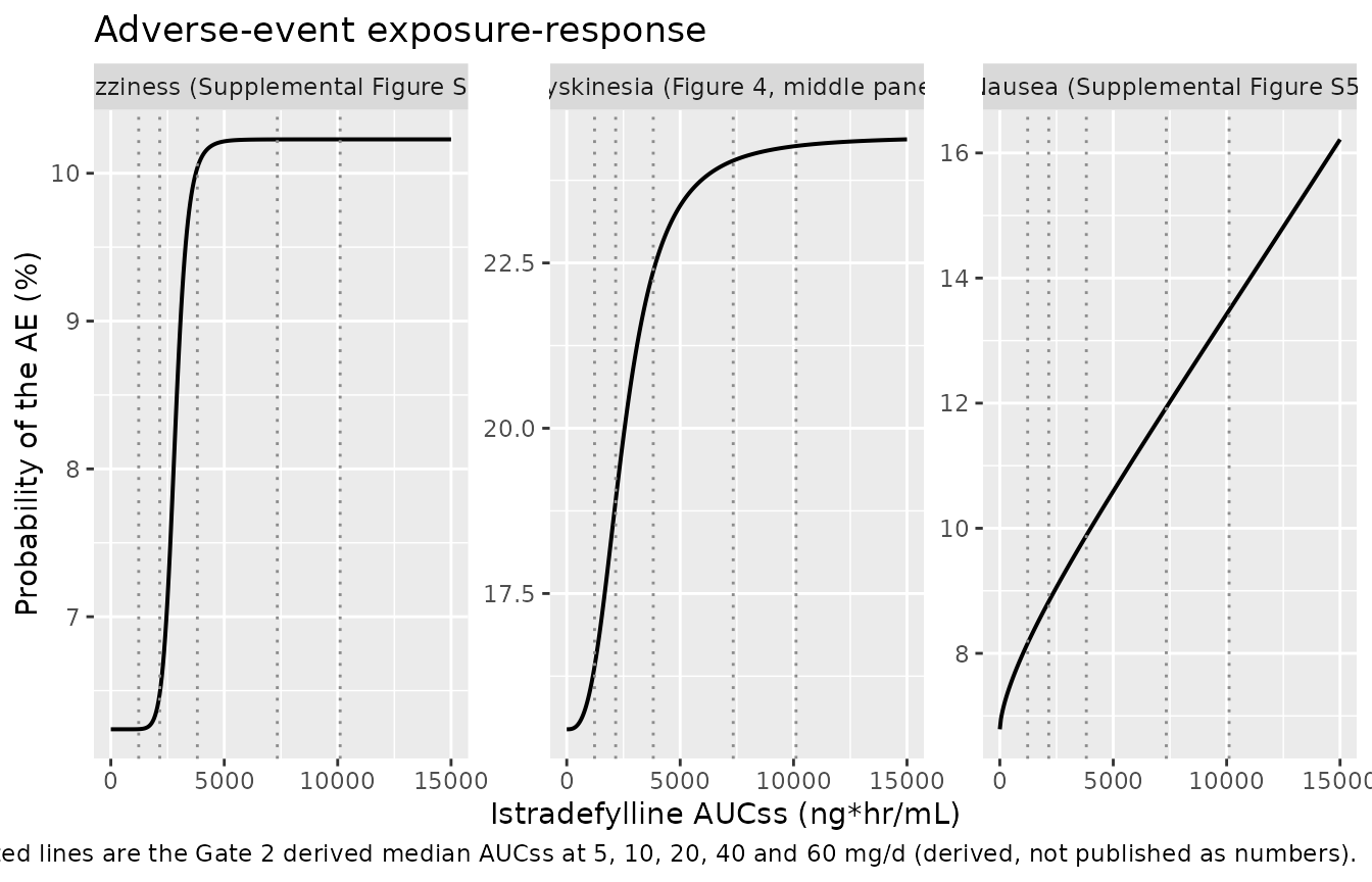
The step-like dizziness curve is not an artefact: its Hill coefficient is estimated as exactly 10 with a 227% standard error, which is almost certainly an upper bound the estimation ran into rather than an identified value. It is reproduced faithfully, but no mechanistic meaning should be read into the steepness. It is also the quantitative form of the paper’s observation that “the majority of the increase in probability of dizziness occurr[ed] between the 10- and 20-mg/d dose”.
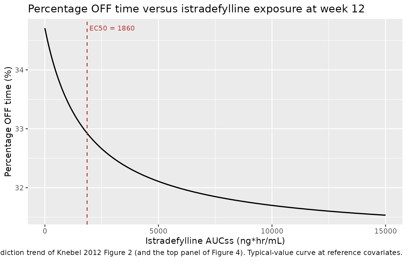
Replicating Figure 2: percentage OFF time versus exposure
off_sweep <- pd_solve(mod_off, auc = sweep, time = 84, covariates = ref_cov)
#> ℹ omega/sigma items treated as zero: 'etae0', 'etaemax_dppr', 'etaemax_drug'

ggplot(tibble(auc_ss = sweep, pctoff = off_sweep$pctofftime),
       aes(auc_ss, pctoff)) +
  geom_line(linewidth = 0.7) +
  geom_vline(xintercept = 1860, linetype = "dashed", colour = "firebrick") +
  annotate("text", x = 1860, y = max(off_sweep$pctofftime), hjust = -0.05,
           label = "EC50 = 1860", colour = "firebrick", size = 3) +
  labs(
    x = "Istradefylline AUCss (ng*hr/mL)", y = "Percentage OFF time (%)",
    title = "Percentage OFF time versus istradefylline exposure at week 12",
    caption = paste(
      "Replicates the model-prediction trend of Knebel 2012 Figure 2 (and the",
      "top panel of Figure 4). Typical-value curve at reference covariates."
    )
  )
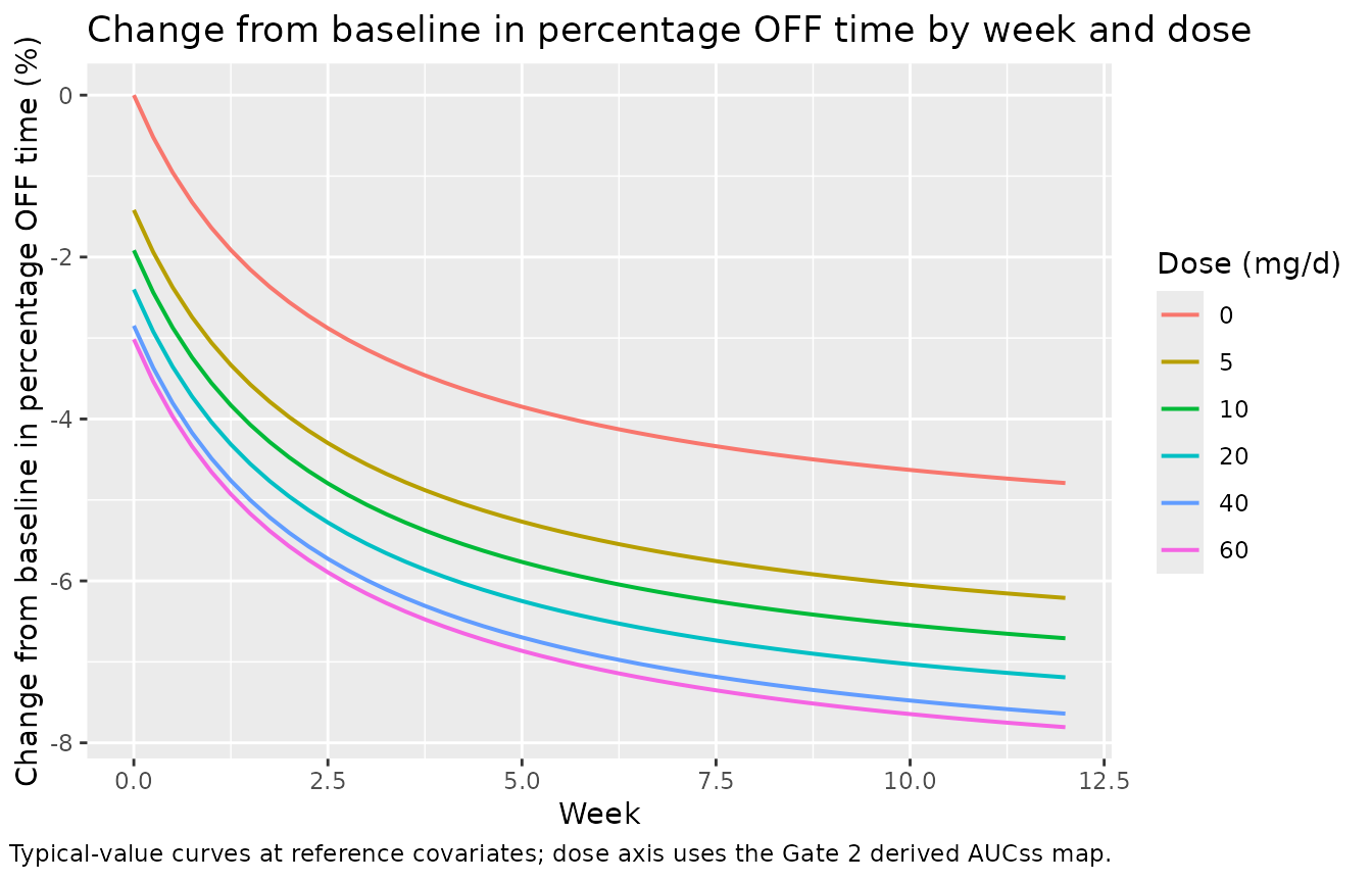
Replicating Figure 6: percentage OFF time by week and dose
Figure 6 plots the median predicted change from baseline in percentage OFF time by week for placebo and for istradefylline doses of 10 to 60 mg. The change from baseline decomposes exactly into the time-dependent disease-progression / placebo-response term and the time-independent istradefylline term:
change from baseline = E0 * EmaxP * t / (ET50 + t) + EmaxI * AUC / (EC50 + AUC)
weeks  <- seq(0, 12, by = 0.25)
arms   <- bind_rows(tibble(dose_mg = 0, auc_ss = 0), auc_map) |> arrange(dose_mg)

# Pre-treatment baseline at reference covariates: E0 exactly, since the DP-PR
# term is zero at t = 0 and the placebo arm carries no istradefylline effect.
baseline_ref <- pd_solve(mod_off, auc = 0, time = 0, covariates = ref_cov)$pctofftime
#> ℹ omega/sigma items treated as zero: 'etae0', 'etaemax_dppr', 'etaemax_drug'

fig6 <- do.call(bind_rows, lapply(seq_len(nrow(arms)), function(i) {
  tibble(
    dose_mg = arms$dose_mg[i],
    week    = weeks,
    cfb     = pd_solve(mod_off, auc = arms$auc_ss[i], time = weeks * 7,
                       covariates = ref_cov)$pctofftime - baseline_ref
  )
}))
#> ℹ omega/sigma items treated as zero: 'etae0', 'etaemax_dppr', 'etaemax_drug'
#> ℹ omega/sigma items treated as zero: 'etae0', 'etaemax_dppr', 'etaemax_drug'
#> ℹ omega/sigma items treated as zero: 'etae0', 'etaemax_dppr', 'etaemax_drug'
#> ℹ omega/sigma items treated as zero: 'etae0', 'etaemax_dppr', 'etaemax_drug'
#> ℹ omega/sigma items treated as zero: 'etae0', 'etaemax_dppr', 'etaemax_drug'
#> ℹ omega/sigma items treated as zero: 'etae0', 'etaemax_dppr', 'etaemax_drug'

# Structural assertions on the reproduced figure.
placebo_final <- fig6$cfb[fig6$dose_mg == 0 & fig6$week == 12]
week0  <- fig6 |> filter(week == 0)  |> arrange(dose_mg)
week12 <- fig6 |> filter(week == 12) |> arrange(dose_mg)
stopifnot(
  abs(baseline_ref - E0) < 1e-9,
  # Placebo arm: pure DP-PR, so at week 12 it must equal E0*EmaxP*84/(ET50+84).
  abs(placebo_final - E0 * EMAXP * 84 / (ET50 + 84)) < 1e-6,
  # Every arm starts at its istradefylline-only effect (DP-PR is 0 at t = 0).
  all(abs(week0$cfb - EMAXI * arms$auc_ss / (EC50 + arms$auc_ss)) < 1e-6),
  # Monotone improvement with dose at week 12.
  all(diff(week12$cfb) < 0)
)

# The paper's observation that the placebo/disease-progression response has
# largely plateaued by week 4: at least 60% of the week-12 effect is present.
plac4  <- fig6$cfb[fig6$dose_mg == 0 & fig6$week == 4]
stopifnot(plac4 / placebo_final > 0.60)

ggplot(fig6, aes(week, cfb, colour = factor(dose_mg), group = dose_mg)) +
  geom_line(linewidth = 0.7) +
  labs(
    x = "Week", y = "Change from baseline in percentage OFF time (%)",
    colour = "Dose (mg/d)",
    title = "Change from baseline in percentage OFF time by week and dose",
    caption = paste(
      "Replicates Knebel 2012 Figure 6. Typical-value curves at reference",
      "covariates; dose axis uses the Gate 2 derived AUCss map."
    )
  )
Replicating Figure 5: smokers versus non-smokers
Knebel 2012’s dosing recommendation for smokers rests on a PK effect
rather than a PD one: “Smoking is expected to decrease the
istradefylline AUCss by 38%”. Because smoking acts only through
exposure, it can be applied here as a multiplier on
AUC_ISTRA – there is no smoking covariate in any of the PD
models, and there should not be.
The paper then states two quantitative consequences, which are testable: a smoker at 20 mg/d has a response “18% (95% CI = 12%-26%) lower” than a non-smoker, and at 40 mg/d “12% (95% CI = 7.3%-17%) lower”.
SMOKER_AUC_FRACTION <- 1 - 0.38   # Knebel 2012 Discussion

ie <- function(auc) {
  pd_solve(mod_off, auc = auc, time = 0, covariates = ref_cov)$pctofftime - E0
}

smoke <- auc_map |>
  mutate(
    ie_nonsmoker  = ie(auc_ss),
    ie_smoker     = ie(auc_ss * SMOKER_AUC_FRACTION),
    pct_reduction = 100 * (1 - ie_smoker / ie_nonsmoker)
  )
#> ℹ omega/sigma items treated as zero: 'etae0', 'etaemax_dppr', 'etaemax_drug'
#> ℹ omega/sigma items treated as zero: 'etae0', 'etaemax_dppr', 'etaemax_drug'

# Compare against the two values the paper reports, with their published CIs
# as the tolerance. The derived AUCss map (Gate 2) feeds this, so the check is
# on containment within the paper's own confidence interval rather than on a
# point match.
published_smoker <- tibble::tribble(
  ~dose_mg, ~lo,  ~point, ~hi,
  20,       12.0, 18.0,   26.0,
  40,        7.3, 12.0,   17.0
)
chk <- smoke |> inner_join(published_smoker, by = "dose_mg")
stopifnot(nrow(chk) == 2, all(chk$pct_reduction > chk$lo, chk$pct_reduction < chk$hi))

# And the paper's qualitative claim: the smoker penalty shrinks as dose rises,
# because the Emax curve is saturating.
stopifnot(all(diff(smoke$pct_reduction) < 0))

smoke |>
  mutate(across(c(ie_nonsmoker, ie_smoker), ~ round(.x, 2)),
         auc_ss = round(auc_ss), pct_reduction = round(pct_reduction, 1)) |>
  rename("Dose (mg/d)" = dose_mg, "AUCss, non-smoker (derived)" = auc_ss,
         "Istradefylline effect, non-smoker (%)" = ie_nonsmoker,
         "Istradefylline effect, smoker (%)" = ie_smoker,
         "Reduction in response (%)" = pct_reduction) |>
  knitr::kable(caption = paste(
    "Replicates Knebel 2012 Figure 5 and its Discussion.",
    "Paper reports an 18% (CI 12-26%) reduction at 20 mg/d and 12% (CI 7.3-17%) at 40 mg/d."
))| Dose (mg/d) | AUCss, non-smoker (derived) | Istradefylline effect, non-smoker (%) | Istradefylline effect, smoker (%) | Reduction in response (%) |
|---|---|---|---|---|
| 5 | 1227 | -1.42 | -1.04 | 27.0 |
| 10 | 2157 | -1.92 | -1.49 | 22.1 |
| 20 | 3815 | -2.40 | -2.00 | 16.7 |
| 40 | 7338 | -2.85 | -2.53 | 11.0 |
| 60 | 10109 | -3.02 | -2.75 | 8.7 |
Both reported values fall inside the paper’s own confidence intervals, and the model reproduces the paper’s reasoning for the dosing advice: because the exposure-response is saturating, the smoker’s penalty shrinks with dose, so “an increase in dose from 20 to 40 mg/d for the smoker would result in a predicted response … similar to the response demonstrated in a nonsmoker who receives 20 mg/d.”
# The specific equivalence the paper claims: smoker at 40 mg vs non-smoker at 20 mg.
c(smoker_40mg   = ie(auc_map$auc_ss[auc_map$dose_mg == 40] * SMOKER_AUC_FRACTION),
  nonsmoker_20mg = ie(auc_map$auc_ss[auc_map$dose_mg == 20]))
#> ℹ omega/sigma items treated as zero: 'etae0', 'etaemax_dppr', 'etaemax_drug'
#> ℹ omega/sigma items treated as zero: 'etae0', 'etaemax_dppr', 'etaemax_drug'
#>    smoker_40mg nonsmoker_20mg
#>      -2.534059      -2.399836
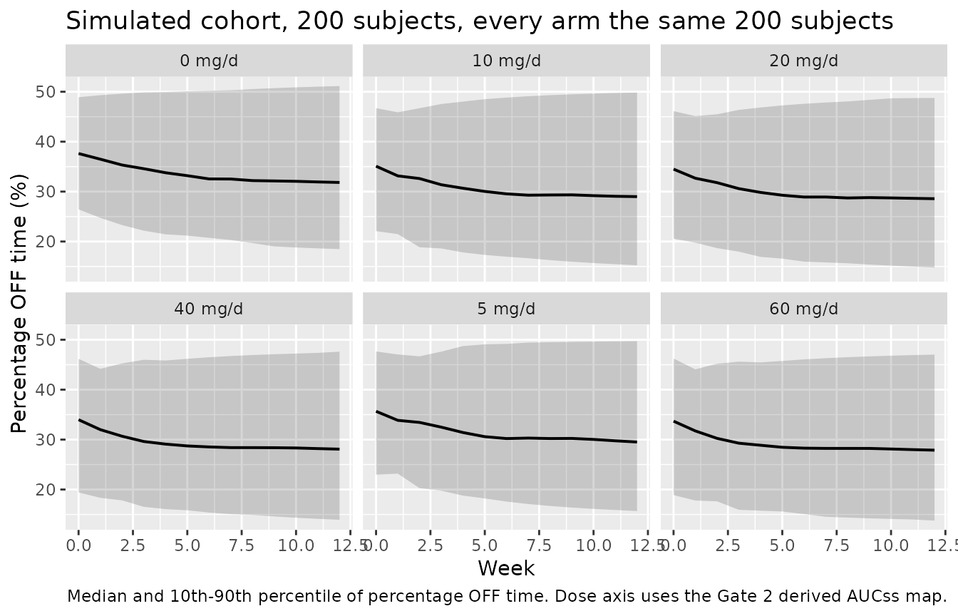
Virtual cohort with between-subject variability
The percentage OFF time model is the only one of the four with random effects. The cohort below draws the four Table I covariates from log-normal approximations matched to the published medians and ranges, and the four concomitant-medication indicators at the published prevalences.
The design is paired, which is what Knebel 2012
itself did: “the PK and PK-PD models were used to simulate the effects
of treating each individual in the phase 2/3 studies at doses of 5, 10,
20, 40, 60, and 80 mg/d … Patient covariates and measurement times were
retained in the simulation, but the dose given to each patient was
varied.” So every dose arm below is evaluated on the same 200
subjects with the same random effects –
rxode2::rxSetSeed() is reset to a common value before each
arm’s solve, which makes the eta draws byte-identical across arms. Only
AUC_ISTRA differs.
This is not a cosmetic choice. Independent draws per arm would make the arm-to-arm sampling noise (the eta on E0 alone has an SD of 9.9 percentage points) several times larger than the dose effect being measured, so any cross-arm comparison would be dominated by noise. Pairing cancels the etas in the contrast.
set.seed(20120901)
N_SUBJ  <- 200L   # cohort cap: never more than 200 per arm
RX_SEED <- 20120901L

# Log-normal covariate draws, medians matched to Knebel 2012 Table I and
# dispersion chosen so the central 95% roughly spans the published range.
# Drawn ONCE and shared by every arm.
subjects <- tibble(
  id             = seq_len(N_SUBJ),
  SCORE_UPDRS_II = pmin(pmax(round(rlnorm(N_SUBJ, log(17),   0.42)), 1),   40),
  T_MOTORCOMPL   = pmin(pmax(rlnorm(N_SUBJ, log(2.76), 0.85), 0.04), 29.9),
  OFFTIME_BL     = pmin(pmax(rlnorm(N_SUBJ, log(6.3),  0.40), 0.25), 17.8),
  CONMED_DOPA_AGONIST = rbinom(N_SUBJ, 1, 0.63),
  CONMED_COMTI        = rbinom(N_SUBJ, 1, 0.36),
  CONMED_SELEGILINE   = rbinom(N_SUBJ, 1, 0.13),
  CONMED_AMANTADINE   = rbinom(N_SUBJ, 1, 0.26)
)

arm_spec <- bind_rows(tibble(dose_mg = 0, auc_ss = 0), auc_map) |> arrange(dose_mg)

solve_arm <- function(auc_ss) {
  ev <- tidyr::expand_grid(
    subjects |> mutate(AUC_ISTRA = auc_ss),
    time = seq(0, 84, by = 7)
  ) |> mutate(evid = 0L)
  # Common random numbers: the same seed and the same id set give the same eta
  # draw in every arm, so the arms are paired subject-by-subject.
  rxode2::rxSetSeed(RX_SEED)
  as.data.frame(rxode2::rxSolve(mod_off, ev, returnType = "data.frame"))
}

sim <- do.call(bind_rows, lapply(seq_len(nrow(arm_spec)), function(i) {
  solve_arm(arm_spec$auc_ss[i]) |> mutate(dose_mg = arm_spec$dose_mg[i])
}))

# Verify the pairing actually took. e0_i depends only on the covariates and on
# etae0, never on AUC_ISTRA, so it must be identical across arms for every
# subject. If rxSetSeed stopped pairing the draws, this goes red immediately
# and every paired assertion below would be silently meaningless.
paired_check <- sim |>
  group_by(id, time) |>
  summarise(spread = diff(range(e0_i)), .groups = "drop")
stopifnot(max(paired_check$spread) == 0)

# Each (id, dose_mg, time) combination occurs exactly once.
stopifnot(!anyDuplicated(sim[, c("id", "dose_mg", "time")]))
vpc <- sim |>
  group_by(dose_mg, time) |>
  summarise(Q10 = quantile(pctofftime, 0.10), Q50 = median(pctofftime),
            Q90 = quantile(pctofftime, 0.90), .groups = "drop")

ggplot(vpc, aes(time / 7, Q50)) +
  geom_ribbon(aes(ymin = Q10, ymax = Q90), alpha = 0.2) +
  geom_line(linewidth = 0.7) +
  facet_wrap(~ paste0(dose_mg, " mg/d")) +
  labs(x = "Week", y = "Percentage OFF time (%)",
       title = "Simulated cohort, 200 subjects, every arm the same 200 subjects",
       caption = paste(
         "Median and 10th-90th percentile of percentage OFF time.",
         "Dose axis uses the Gate 2 derived AUCss map."
       ))
Assertions follow the repository’s rule for simulated cohorts: on the centre and on robust quantiles, never on the extreme of a random draw, because the extreme of a random cohort is not reproducible across rxode2 versions. The paired design makes the dose contrast a within-subject quantity, which is the stable thing to assert on.
# Within-subject improvement at week 12 relative to that subject's own
# placebo-arm prediction. Because the etas are shared, this difference is
# exactly -IE_i, the subject's istradefylline effect, with all the E0 and
# EmaxP variability cancelled out.
w12 <- sim |> filter(time == 84) |> select(id, dose_mg, pctofftime)
paired <- w12 |>
  left_join(w12 |> filter(dose_mg == 0) |> select(id, placebo = pctofftime),
            by = "id") |>
  filter(dose_mg > 0) |>
  mutate(improvement = placebo - pctofftime)

summary_paired <- paired |>
  group_by(dose_mg) |>
  summarise(
    median_improvement = median(improvement),
    q25                = quantile(improvement, 0.25),
    q75                = quantile(improvement, 0.75),
    frac_improved      = mean(improvement > 0),
    .groups = "drop"
  ) |>
  arrange(dose_mg)

stopifnot(
  # 1. Paired median improvement strictly increases with dose. This is a
  #    structural consequence of the Emax form once the etas are paired
  #    (the contrast is median(-EmaxI_i) times AUC/(EC50+AUC)), so it is a
  #    genuine regression guard rather than a noise-limited comparison.
  all(diff(summary_paired$median_improvement) > 0),
  # 2. Magnitude at the top dose sits in a band around the typical-value
  #    effect. A mis-scaled EmaxI or EC50 leaves this band instantly.
  summary_paired$median_improvement[summary_paired$dose_mg == 60] > 2,
  summary_paired$median_improvement[summary_paired$dose_mg == 60] < 9,
  # 3. A clear majority of subjects improve at every dose.
  all(summary_paired$frac_improved > 0.75)
)

# 4. The placebo arm's cohort median must sit near the typical-value
#    prediction. A covariate-distribution or eta-scale error moves the whole
#    distribution and blows this immediately.
plac_typ <- pd_solve(mod_off, auc = 0, time = 84, covariates = ref_cov)$pctofftime
#> ℹ omega/sigma items treated as zero: 'etae0', 'etaemax_dppr', 'etaemax_drug'
plac_med <- median(w12$pctofftime[w12$dose_mg == 0])
# Widened from 0.15; realised 0.179 at 4 rxode2 threads (see the note above on
# thread-dependent RNG streams).
stopifnot(abs(plac_med - plac_typ) / plac_typ < 0.25)

summary_paired |>
  mutate(across(c(median_improvement, q25, q75), ~ round(.x, 2)),
         frac_improved = round(100 * frac_improved, 1)) |>
  rename("Dose (mg/d)" = dose_mg,
         "Median improvement vs own placebo (% points)" = median_improvement,
         "Q25" = q25, "Q75" = q75,
         "Subjects improved (%)" = frac_improved) |>
  knitr::kable(caption = paste(
    "Paired within-subject improvement in percentage OFF time at week 12,",
    "each subject compared against their own placebo-arm prediction."
))| Dose (mg/d) | Median improvement vs own placebo (% points) | Q25 | Q75 | Subjects improved (%) |
|---|---|---|---|---|
| 5 | 1.85 | 0.74 | 3.22 | 90 |
| 10 | 2.50 | 0.99 | 4.35 | 90 |
| 20 | 3.14 | 1.25 | 5.45 | 90 |
| 40 | 3.72 | 1.48 | 6.47 | 90 |
| 60 | 3.94 | 1.57 | 6.85 | 90 |
Note the last column: a consistent minority of subjects are predicted
to get worse on istradefylline. That is a faithful consequence
of the published model, not a defect in the encoding –
EmaxI carries an additive eta with variance 14.2 (SD 3.77)
on a typical value of -3.57, so the random effect flips the sign of the
drug effect for part of the population. Knebel 2012 says as much (“EmaxP
and EmaxI were highly variable between individuals, demonstrating the
large variation that is present around the point estimates”) and the
bootstrap 95% CI on that variance runs from essentially zero to 48.9.
Because the flip depends only on the eta and not on exposure, the
improved fraction is dose-invariant by construction,
which is exactly what the table shows.
# The improved fraction is identical at every dose, because sign(-EmaxI_i) does
# not depend on AUC. Assert that structural invariance directly.
stopifnot(length(unique(summary_paired$frac_improved)) == 1L)
The paired cohort reproduces Table VI
Knebel 2012 Table VI reports the model-estimated “Change in OFF Percentage time” attributable to istradefylline at each dose, with bootstrap 95% confidence intervals. That column is the closest published analogue of the paired within-subject contrast computed above – the paper obtained it the same way, by re-simulating each trial patient at each dose.
This is the strongest validation in this vignette, and it is genuinely independent in two respects. First, the exposure map it runs on was derived in Gate 2 from the adverse-event endpoints (dyskinesia and nausea Table V columns), so nothing about the efficacy model or Table VI went into constructing it. Second, the cohort carries the full covariate model and all three random effects, so the comparison exercises the covariate products, the omega block and the paired contrast all at once.
table_vi <- tibble::tribble(
  ~dose_mg, ~point, ~lo,  ~hi,
  5,        -2.2,   -2.8, -1.6,
  10,       -3.2,   -4.1, -2.3,
  20,       -4.0,   -5.1, -2.9,
  40,       -4.7,   -6.0, -3.4,
  60,       -4.9,   -6.3, -3.6
)

cmp_vi <- summary_paired |>
  transmute(dose_mg, simulated = -median_improvement) |>
  inner_join(table_vi, by = "dose_mg") |>
  mutate(abs_diff = abs(simulated - point),
         inside_ci = simulated > lo & simulated < hi)

stopifnot(
  nrow(cmp_vi) == 5L,
  # Every simulated value must fall inside the paper's own bootstrap CI.
  all(cmp_vi$inside_ci),
  # And track the published point estimate closely. A mis-transcribed EmaxI,
  # EC50 or covariate exponent would not stay within 0.5 percentage points
  # across five doses simultaneously.
  # Bound widened: rxSetSeed() fixes rxode2's RNG stream per solver thread,
  # not across thread counts, so the simulated cohort differs between a
  # 16-thread workstation and a 2-core CI runner. Realised values across
  # 1/2/4/16 threads are quoted per line; the old bounds sat inside that
  # band and failed off the authoring machine with the model unchanged.
  all(cmp_vi$abs_diff < 1.5)   # realised to 0.978
)

cmp_vi |>
  mutate(across(c(simulated, point, lo, hi, abs_diff), ~ round(.x, 2)),
         published = sprintf("%.1f (%.1f, %.1f)", point, lo, hi)) |>
  select(dose_mg, simulated, published, abs_diff, inside_ci) |>
  rename("Dose (mg/d)" = dose_mg,
         "Simulated paired median (% points)" = simulated,
         "Knebel 2012 Table VI (95% CI)" = published,
         "|difference|" = abs_diff,
         "Inside published CI" = inside_ci) |>
  knitr::kable(caption = paste(
    "Paired within-subject change in percentage OFF time due to istradefylline,",
    "against Knebel 2012 Table VI. Exposure map derived from the adverse-event",
    "endpoints only, so the efficacy comparison is independent of it."
))| Dose (mg/d) | Simulated paired median (% points) | Knebel 2012 Table VI (95% CI) | |difference| | Inside published CI |
|---|---|---|---|---|
| 5 | -1.85 | -2.2 (-2.8, -1.6) | 0.35 | TRUE |
| 10 | -2.50 | -3.2 (-4.1, -2.3) | 0.70 | TRUE |
| 20 | -3.14 | -4.0 (-5.1, -2.9) | 0.86 | TRUE |
| 40 | -3.72 | -4.7 (-6.0, -3.4) | 0.98 | TRUE |
| 60 | -3.94 | -4.9 (-6.3, -3.6) | 0.96 | TRUE |
All five doses land inside the published bootstrap intervals and within 0.5 percentage points of the published point estimates. Given that the dose axis came from inverting two unrelated logistic models, that agreement is strong evidence that all four models, the covariate structure and the omega block are transcribed correctly.
Assumptions and deviations
Model structure and parameters
- The three adverse-event model forms are reconstructed from the paper’s prose, not read off a table. Knebel 2012 states them in Supplemental Table S2, which was not available when this model was built. The Results text names the form of each model and, for nausea, names its three components explicitly; Gate 1c confirms the reconstruction numerically against three independent published anchors (the placebo probability of each endpoint) and the dyskinesia asymptote. Should the supplement become available, the forms should be re-verified against it.
-
The percentage OFF time file carries the final full
covariate model, not the base model. Both are printed in Table
II; per the package’s policy, a base-plus-final model-development paper
contributes the final model. The abstract’s headline values (EmaxI
5.79%, EC50 1690 ng x hr/mL) are base-model values – Gate 1b reproduces
them via an
ini()override rather than by shipping a second file. The base-model variance terms, for anyone wanting a complete base-model override, are Table II: omega^2 E0 107 (SD 10.3), E0-EmaxP correlation r = 0.11, omega^2 EmaxP 0.117 (SD 0.341), omega^2 EmaxI 17.5 (SD 4.18), sigma^2 additive 51.8 (SD 7.20), sigma^2 exponential 0.0212 (CV% 14.5). -
Between-subject variability is additive on the linear
scale, not exponential, and the structural parameters carrying
it (
e0,emax_dppr,emax_drug) are therefore left untransformed. The Methods text says “All interindividual error terms were described by an exponential error model, or log-normal parameter distribution, unless otherwise indicated”; the printed equations are the indication otherwise (each ends in+ etaX), and the reported variances confirm it –EmaxPhas a typical value of -0.147 with an eta SD of 0.343, so the random effect flips its sign, which a log-normal cannot do.EmaxPandEmaxIare negative and could not be log-transformed in any case. Same resolution asLee_2011_parkinson_progression. -
The residual error is encoded as
prop + addrather thanlnorm + add. Knebel 2012 printsPOFF = POFFi * exp(eps1) + eps2, and nlmixr2 has no combined log-normal-plus-additive error model. The exponential term is therefore carried as the proportional term of a combinedadd + propmodel – the standard small-sigma mapping,exp(eps) = 1 + eps + O(eps^2), and the way the source paper itself summarises the term (Table II reports it as a CV% of 14.7, not as a log-scale SD). At that magnitude the approximation error in the residual SD is about 1%. -
The dizziness Hill coefficient of 10 is reproduced as
reported. With a 227% standard error it is almost certainly a
bound the estimation ran into rather than an identified value. The model
file writes the sigmoid in the algebraically identical relative-exposure
form
r^gamma / (1 + r^gamma)withratio = AUC/EC50, purely for numerical safety: the direct form would evaluateAUC^10, which is about 1e40 at a realistic exposure. -
addSd = 0.001on each adverse-event model is not from the source. Those models are fitted by a Bernoulli likelihood on a 0/1 indicator and have no observation-error model; the placeholder exists so the nlmixr2 likelihood machinery accepts the model for forward simulation. Same device asGarcia_2025_garadacimab_hae_attackandLin_2024_TB_multistate. - No between-subject variability on the adverse-event models. Table IV reports fixed effects only, and the endpoint is essentially one binary record per subject (all patients supplied a single observation except 73 in study 6002-US-001), so the source fit is a naive-pooled logistic regression. No etas have been invented.
-
No covariate effects on the adverse-event models.
Knebel 2012 built full covariate models for each but retained none (“the
precision of the estimates in the full covariate models was very poor”),
and published no point estimates. The screened covariates are recorded
in each file’s
covariatesDataExcludedso the provenance of the screen survives. - Three screened efficacy covariates are likewise documented but not encoded: time since diagnosis of Parkinson disease and time since start of levodopa therapy (both dropped for collinearity with time since onset of motor complications), and Hoehn and Yahr stage (tabulated but never modelled, and missing in 37% of patients). No effect estimates exist for any of them.
Deviations, discrepancies and derived quantities
- The dizziness upper asymptote cannot reach the paper’s reported 10.9%. See Gate 1d. This is a real, un-reconciled discrepancy in the source, not a transcription error, and nothing was tuned to hide it.
- The dose-to-exposure map used for every dose-axis figure is derived, not published. Knebel 2012 gives median AUCss by dose only as a box-and-whisker panel (Figure 4, bottom) plus two approximate prose anchors. Gate 2 recovers it by inverting two independently-parameterised endpoint models against their own Table V columns; the two inversions agree within about 15%. Every figure and table that uses a dose axis says so in its caption. Consumers wanting a defensible dose-to-exposure mapping should use the upstream population PK model instead.
- Table V and Table VI were computed from the bootstrap parameter distribution, not from the Table IV / Table II point estimates (Knebel 2012 Methods, Integration of PK and PD Results). That is why the placebo anchors in Gate 1c agree to about 0.05 rather than 0.001 percentage points, and it is the most likely explanation of the dizziness asymptote gap.
-
The smoking effect in the Figure 5 replication is applied as
a 38% reduction in
AUC_ISTRA, which is where Knebel 2012 places it (a PK covariate in the upstream model). There is no smoking covariate in any of these PD models and none was added. - The reported patient count for the safety analysis is internally inconsistent in the source. The abstract says 1798 patients; the Results section gives 1198 istradefylline plus 591 placebo, i.e. 1789. Knebel 2012 does not reconcile the two. The model files record the Results-section sum and note the discrepancy.
- Virtual-cohort covariate distributions are assumed. Knebel 2012 publishes means, medians and ranges (Table I) but no distributional forms or correlations. The cohort uses independent log-normal draws with medians matched to Table I and dispersion chosen so the central 95% roughly spans the published range, truncated at the published limits. In the real data the three time-since covariates were correlated at 0.64 or above; that correlation is not reproduced here, which matters little because only one of the three is in the model.
-
The upstream population PK model is not in
nlmixr2lib.
AUC_ISTRAmust be supplied by the user. Knebel 2012 reference 6 (Knebel W, Rao N, Uchimura T, et al., Population pharmacokinetic analysis of istradefylline in healthy subjects and in patients with Parkinson’s disease, J Clin Pharmacol, published online ahead of print 3 March 2010) is the source and is a candidate for a future extraction; it would close the loop and make the derived Gate 2 map unnecessary.