Paracetamol with hepatic-pathway maturation (Wu 2025)
Source:vignettes/articles/Wu_2025_paracetamol.Rmd
Wu_2025_paracetamol.Rmd
library(nlmixr2lib)
library(PKNCA)
#>
#> Attaching package: 'PKNCA'
#> The following object is masked from 'package:stats':
#>
#>     filter
library(rxode2)
#> rxode2 5.1.2 using 2 threads (see ?getRxThreads)
#>   no cache: create with `rxCreateCache()`
library(dplyr)
#>
#> Attaching package: 'dplyr'
#> The following objects are masked from 'package:stats':
#>
#>     filter, lag
#> The following objects are masked from 'package:base':
#>
#>     intersect, setdiff, setequal, union
library(tidyr)
library(ggplot2)
Model and source
- Citation: Wu Y, Voller S, Goulooze SC, Allegaert K, Sherwin CMT, van Rongen A, Roofthooft DWE, Simons SHP, Tibboel D, Flint RB, van den Anker JN, Knibbe CAJ (2025). A Novel Maturation Equation for Hepatic Clearance Across Preterm, Term Neonates, Children, and Adults: Application to Paracetamol and Its Metabolite. J Clin Pharmacol 65(12):1829-1843. doi:10.1002/jcph.70080. GFR-maturation backbone reproduced from Wu Y et al. Pharm Res 2024;41:637-649 (doi:10.1007/s11095-024-03677-3). Rectal-absorption parameters (Ka, Tlag, F) reproduced from Wang C et al. J Clin Pharmacol 2014;54(6):619-629 (doi:10.1002/jcph.259).
- Description: Parent-and-three-metabolites population PK model for intravenous and rectal paracetamol (PCM) and its glucuronide (PCM-GLU), sulfate (PCM-SULF), and combined oxidative metabolites (PCM-cysteine + PCM-mercapturate, PCM-OXI, denoted with the canonical cysmer suffix) from preterm and term neonates through infants, children, and adults (Wu 2025). Two-compartment plasma disposition for parent PCM with three parallel formation clearances and parallel renal elimination of unchanged parent; one-compartment plasma disposition for each metabolite with renal elimination expressed as a fraction of glomerular filtration rate (GFR). The preterm-and-term-neonate-to-adult (PTNA) maturation equation (Wu 2024) is applied to each formation clearance and to a separate PCM-SULF renal-secretion clearance; an additional adult-only correction factor scales the renal clearance of PCM-GLU in subjects >= 18 years. Rectal absorption parameters (Ka, Tlag, F) are fixed from Wang 2014.
- Article: https://doi.org/10.1002/jcph.70080
- GFR-maturation backbone (parameters fixed from this prior publication): https://doi.org/10.1007/s11095-024-03677-3
- Rectal-absorption Ka / Tlag / F backbone (parameters fixed from this prior publication): https://doi.org/10.1002/jcph.259
Population
Wu et al. (2025) pooled plasma and urine paracetamol (PCM) and
metabolite concentration-time data from 298 subjects across eight
studies, ranging from preterm neonates of 23 weeks gestational age (GA)
and 460 g to healthy adults (50 years, 91.7 kg). The neonatal subset
(datasets 1-5, n = 235) provided gestational age, birthweight, postnatal
age (PNA), and current weight; the infant / child / adult subset
(datasets 6-8, n = 63) used a uniform 40-week GA assumption because the
true GA was not recorded. Of the 6428 observations, the neonatal
datasets contributed both plasma and urine measurements while datasets
6, 7, and 8 contributed plasma data only (with full urine sampling in
three of the neonatal studies for direct estimation of formation and
renal-elimination clearances). The same population description is
available programmatically via
readModelDb("Wu_2025_paracetamol")$population after the
model is loaded.
Source trace
Per-parameter origins are in the in-file comments of
inst/modeldb/specificDrugs/Wu_2025_paracetamol.R. The
compact summary below collects the structural equations and key fixed /
estimated parameters.
| Equation / parameter | Value | Source location |
|---|---|---|
| Two-cpt PCM + one-cpt per metabolite + rectal depot | n/a | Methods “Base Model” (p. 1833) |
| Volume scaling reference (PCM disposition) | 1080 g (= 1.08 kg) | Table 3 “Paracetamol” block |
| Birth / current weight reference (formation CL, GFR) | 1750 g (= 1.75 kg) | Table 3 formation-CL rows; Wu 2024 GFR equation |
lvp typical V_P |
1.01 L | Table 3 TVvp |
e_wt_vp allometric exponent on V_P |
0.9781 | Table 3 theta_BWc(V_P) |
lvpp typical V_PP |
0.2707 L | Table 3 TVvpp |
e_wt_vpp exponent on V_PP (fixed 0) |
0 | Table 3 (FIXED) |
lq typical Q |
0.08921 L/h | Table 3 TVQ |
e_wt_q allometric exponent on Q |
2.212 | Table 3 theta_BWc(Q) |
lka, ltlag, lfdepot
(rectal) |
0.275 /h, 0.0103 h, 0.96 | Table 3, fixed from Wang 2014 |
| PTNA equation (formation CL) | per metabolite | Methods “PTNA Equation” / Eq. 8 |
lclbirth_gluc, lclmax_gluc,
lpna50_gluc, e_ga_pna50_gluc,
lhill_gluc
|
0.007961 / 0.3378 L/h / 62.67 d / -4.625 / 1.553 | Table 3 PCM-GLU block |
lclbirth_sulf, lclmax_sulf,
lpna50_sulf, lhill_sulf
|
0.1854 / 0.3787 L/h / 25.92 d / 1.955 | Table 3 PCM-SULF block (no-GA, theta_GAPNA50 = 0 FIXED) |
lclbirth_cysmer, lclmax_cysmer,
lpna50_cysmer, lhill_cysmer
|
0.02047 / 0.06377 L/h / 10.47 d / 2.972 | Table 3 PCM-OXI block (no-GA, theta_GAPNA50 = 0 FIXED) |
GFR PTNA: lclbirth_gfr, lclmax_gfr,
e_wt_gfr, lpna50_gfr,
e_ga_pna50_gfr, lhill_gfr
|
1.26 / 8.98 mL/min, 0.738, 34 d, -3.61, 1.03 | Wu 2024 Eq. 1 (FIXED) – mL/min pre-converted to L/h via x0.06 |
lfrn_pcm, lfrn_gluc,
lf_gluc_adult, lfrn_sulf,
lfrn_cysmer
|
0.08486 / 0.4475 / 1.663 / 0.3059 / 0.7393 | Table 3 renal-elimination block |
PCM-SULF secretion (simplified PTNA, Hill = 1, CL_birth = 0):
lclmax_secr_sulf, lpna50_secr_sulf,
e_ga_pna50_secr_sulf
|
11.92 mL/min, 80.03 d, -5.849 | Table 3 secretion sub-block (mL/min unit convention inherited from GFR) |
Metabolite volume fractions: lf_vol_gluc,
lf_vol_sulf, lf_vol_cysmer
|
0.3299 / 0.3476 / 0.7048 | Table 3 “Volume of distribution” block (V_G, V_S, V_O = fraction x V_P) |
Plasma residual SDs: propSd, propSd_gluc,
propSd_sulf, propSd_cysmer
|
0.2657 / 0.5101 / 0.2866 / 0.3947 | Table 3 residual-variance rows (variance reported – SD = sqrt(variance)) |
Virtual cohort: four typical individuals
Wu et al. (2025) Figures 3 and 4 simulate four typical individuals born with GA of 26, 30, 35, and 40 weeks (corresponding birthweights 850, 1350, 2450, and 3500 g) followed from birth to 18 years. To reproduce these typical-individual curves we evaluate the model at a dense PNA grid for each (GA, birthweight) pair, with current weight following a smooth piecewise interpolation from birthweight (PNA = 0) through pediatric growth to the adult typical weight of 70 kg.
# Piecewise interpolation of current weight (kg) vs postnatal age (months).
# Anchors approximate WHO weight-for-age curves (term reference) extended through
# adolescence to a 70 kg adult; the same anchor shape is used for every cohort
# (a single Wu 2025-Figure 3 simulation track per GA + birthweight pair).
weight_anchors_months <- c(0, 1, 3, 6, 12, 24, 60, 12*10, 12*15, 12*18)
weight_anchors_kg     <- c(NA, 3.8, 6.0, 7.5, 10.0, 12.5, 19.0, 32.0, 55.0, 70.0)

typical_weight <- function(birthweight_kg, PNA_months) {
  anchors_kg <- weight_anchors_kg
  anchors_kg[1] <- birthweight_kg
  approx(weight_anchors_months, anchors_kg, xout = PNA_months, rule = 2)$y
}

# Four typical individuals from Wu 2025 Methods (Model Simulation).
typical_subjects <- tibble::tribble(
  ~cohort,    ~GA,  ~WT_BIRTH,
  "GA 26 wk", 26L,  0.850,
  "GA 30 wk", 30L,  1.350,
  "GA 35 wk", 35L,  2.450,
  "GA 40 wk", 40L,  3.500
)
Simulation: clearance maturation for the four typical individuals
mod <- readModelDb("Wu_2025_paracetamol")
mod_typical <- mod |> rxode2::zeroRe()
#> ℹ parameter labels from comments will be replaced by 'label()'

# Build the event table: one observation row per cohort at each PNA grid
# point. PNA from 1 day (0.0329 months) to 18 years (216 months) on a log-
# spaced grid; a single zero-amount dose at the start anchors the integrator.
pna_grid_months <- exp(seq(log(1 / 30.4375), log(18 * 12), length.out = 80))

events_maturation <- typical_subjects |>
  dplyr::mutate(id = dplyr::row_number()) |>
  tidyr::crossing(time_h = c(0, pna_grid_months * 30.4375 * 24)) |>
  dplyr::mutate(
    PNA  = time_h / 24 / 30.4375,           # current PNA at each observation (months)
    WT   = typical_weight(WT_BIRTH, PNA),
    evid = ifelse(time_h == 0, 1L, 0L),     # token dose at t = 0 to anchor solver
    amt  = ifelse(time_h == 0, 1, 0),       # 1 mg token IV dose; we only use derived CL columns
    cmt  = ifelse(evid == 1L, "central", "Cc"),
    time = time_h
  ) |>
  dplyr::select(id, cohort, time, evid, amt, cmt, WT, WT_BIRTH, GA, PNA)
#> Warning: There was 1 warning in `dplyr::mutate()`.
#> ℹ In argument: `WT = typical_weight(WT_BIRTH, PNA)`.
#> Caused by warning in `anchors_kg[1] <- birthweight_kg`:
#> ! number of items to replace is not a multiple of replacement length

sim_maturation <- rxode2::rxSolve(
  mod_typical, events = events_maturation,
  keep = c("cohort", "GA", "WT_BIRTH")
) |>
  as.data.frame() |>
  dplyr::filter(time > 0) |>                # drop the anchor row
  dplyr::mutate(
    PNA_years    = time / 24 / 30.4375 / 12,
    cl_form_pcm  = cl_form_gluc + cl_form_sulf + cl_form_cysmer,
    cl_total     = cl_form_pcm + cl_renal_pcm,
    f_gluc       = cl_form_gluc   / cl_total,
    f_sulf       = cl_form_sulf   / cl_total,
    f_cysmer     = cl_form_cysmer / cl_total,
    f_renal_pcm  = cl_renal_pcm   / cl_total
  )
#> ℹ omega/sigma items treated as zero: 'etalvp', 'etalka', 'etalcl_gluc', 'etalcl_sulf', 'etalcl_cysmer', 'etalfrn_pcm', 'etalfrn_gluc', 'etalfrn_sulf', 'etalfrn_cysmer'
#> Warning: multi-subject simulation without without 'omega'
Figure 3 reproduction – absolute CL by pathway vs PNA
Wu et al. (2025) Figure 3: total PCM CL and the four elimination-pathway CLs (GLU formation, SULF formation, OXI formation, and renal CL of unchanged PCM) versus postnatal age for four typical individuals.
cl_long <- sim_maturation |>
  dplyr::select(PNA_years, cohort,
                `Total PCM`     = cl_total,
                `Glucuronidation` = cl_form_gluc,
                `Sulfation`     = cl_form_sulf,
                `Oxidation`     = cl_form_cysmer,
                `Renal CL PCM`  = cl_renal_pcm) |>
  tidyr::pivot_longer(c(-PNA_years, -cohort),
                      names_to = "Pathway", values_to = "CL_Lh") |>
  dplyr::mutate(
    Pathway = factor(Pathway, levels = c("Total PCM", "Glucuronidation",
                                         "Sulfation", "Oxidation", "Renal CL PCM"))
  )

ggplot(cl_long, aes(x = PNA_years, y = CL_Lh, color = cohort)) +
  geom_line(linewidth = 0.8) +
  scale_x_log10(breaks = c(1/365, 7/365, 1/12, 1, 5, 18),
                labels = c("1 d", "1 w", "1 mo", "1 yr", "5 yr", "18 yr")) +
  scale_y_log10() +
  facet_wrap(~Pathway, scales = "free_y") +
  labs(x = "Postnatal age", y = "Clearance (L/h)",
       color = "Birth cohort",
       caption = "Replicates Figure 3 of Wu 2025.") +
  theme_bw() +
  theme(legend.position = "bottom")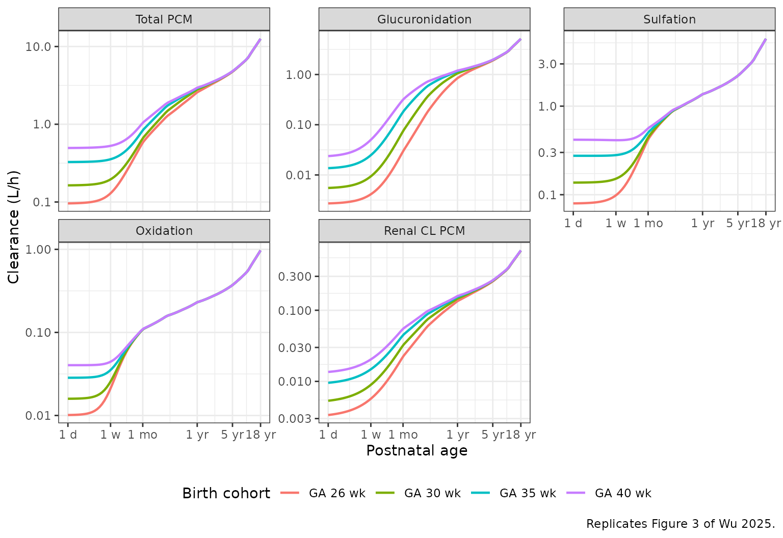
Figure 4 reproduction – pathway fractions vs PNA
Wu et al. (2025) Figure 4: fraction of total PCM CL contributed by each pathway versus postnatal age, for the same four typical individuals.
frac_long <- sim_maturation |>
  dplyr::select(PNA_years, cohort,
                `Glucuronidation`     = f_gluc,
                `Sulfation`           = f_sulf,
                `Oxidation`           = f_cysmer,
                `Renal CL PCM`        = f_renal_pcm) |>
  tidyr::pivot_longer(c(-PNA_years, -cohort),
                      names_to = "Pathway", values_to = "fraction") |>
  dplyr::mutate(
    Pathway = factor(Pathway, levels = c("Sulfation", "Glucuronidation",
                                         "Oxidation", "Renal CL PCM"))
  )

ggplot(frac_long, aes(x = PNA_years, y = fraction, color = cohort)) +
  geom_line(linewidth = 0.8) +
  scale_x_log10(breaks = c(1/365, 7/365, 1/12, 1, 5, 18),
                labels = c("1 d", "1 w", "1 mo", "1 yr", "5 yr", "18 yr")) +
  scale_y_continuous(limits = c(0, 1), labels = scales::percent) +
  facet_wrap(~Pathway, ncol = 2) +
  labs(x = "Postnatal age",
       y = "Fraction of total PCM CL",
       color = "Birth cohort",
       caption = "Replicates Figure 4 of Wu 2025.") +
  theme_bw() +
  theme(legend.position = "bottom")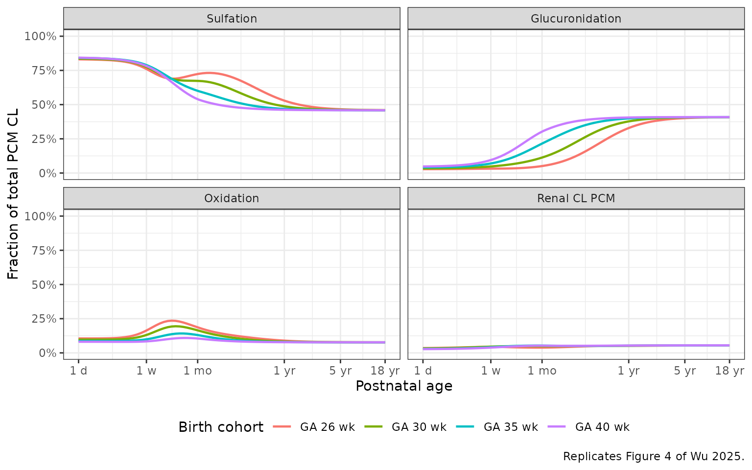
Sanity checks against the paper’s narrative (Results, Model Simulation):
- At 1 month of age, glucuronidation contributes ~5% of total PCM CL in the 26-week preterm cohort and ~30% in the term cohort.
- Sulfation accounts for ~80% of total PCM CL at birth and falls to ~45% in adulthood.
- Oxidation begins at ~8-11% at birth and stabilises near 8% in adults.
milestones <- sim_maturation |>
  dplyr::filter(PNA_years > 1/12 * 0.99 & PNA_years < 1/12 * 1.01 |
                PNA_years > 18 * 0.99   & PNA_years < 18 * 1.01) |>
  dplyr::mutate(milestone = ifelse(PNA_years < 1, "1 month", "18 years")) |>
  dplyr::group_by(milestone, cohort) |>
  dplyr::summarise(
    f_gluc_pct       = round(100 * mean(f_gluc), 1),
    f_sulf_pct       = round(100 * mean(f_sulf), 1),
    f_cysmer_pct     = round(100 * mean(f_cysmer), 1),
    f_renal_pcm_pct  = round(100 * mean(f_renal_pcm), 1),
    .groups = "drop"
  )
knitr::kable(milestones, caption = "Pathway fractions at 1 month and 18 years (typical individuals).")| milestone | cohort | f_gluc_pct | f_sulf_pct | f_cysmer_pct | f_renal_pcm_pct |
|---|---|---|---|---|---|
| 18 years | GA 26 wk | 40.8 | 46.0 | 7.7 | 5.5 |
| 18 years | GA 30 wk | 40.9 | 45.9 | 7.7 | 5.5 |
| 18 years | GA 35 wk | 40.9 | 45.9 | 7.7 | 5.5 |
| 18 years | GA 40 wk | 40.9 | 45.9 | 7.7 | 5.5 |
Simulation: adult PK profile after a single 2000 mg IV PCM dose
Reproduce the adult Dataset 8 dosing regimen (initial 2000 mg PCM over 20 min, followed by 1000 mg every 6 h post-protocol) to support a single-dose NCA validation. The published adult cohort is small (n = 8 healthy adults 18-50 years, 53.4-91.7 kg) so a virtual cohort of 50 adults is used to characterise the simulated central tendency.
set.seed(70080)
n_adult <- 50

adults <- tibble::tibble(
  id        = seq_len(n_adult),
  cohort    = "Adult 2 g IV",
  WT        = rnorm(n_adult, mean = 70, sd = 12),
  WT_BIRTH  = 3.5,
  GA        = 40,
  PNA       = 30 * 12     # 30 years in months -- well above the 18-year adult cutoff
) |>
  dplyr::mutate(WT = pmax(45, pmin(WT, 110)))

# 2000 mg IV bolus at t = 0 (the paper used a 20-min infusion of two 1000 mg
# doses; for NCA we use a single bolus into central -- the AUC is preserved).
dose_adult <- adults |>
  dplyr::transmute(
    id, cohort, time = 0, evid = 1L, amt = 2000, cmt = "central",
    WT, WT_BIRTH, GA, PNA
  )

obs_times <- c(0.05, seq(0.25, 24, by = 0.5))
obs_adult <- adults |>
  tidyr::crossing(time = obs_times) |>
  dplyr::mutate(evid = 0L, amt = 0, cmt = "Cc")

events_adult <- dplyr::bind_rows(dose_adult, obs_adult) |>
  dplyr::arrange(id, time, dplyr::desc(evid))

sim_adult <- rxode2::rxSolve(
  mod, events = events_adult,
  keep      = c("cohort", "WT", "WT_BIRTH", "GA", "PNA")
) |>
  as.data.frame()
#> ℹ parameter labels from comments will be replaced by 'label()'
Adult PK profile
adult_quant <- sim_adult |>
  dplyr::filter(time > 0) |>
  dplyr::select(time,
                PCM         = Cc,
                Glucuronide = Cc_gluc,
                Sulfate     = Cc_sulf,
                Cysmer      = Cc_cysmer) |>
  tidyr::pivot_longer(-time, names_to = "Species", values_to = "Conc") |>
  dplyr::group_by(time, Species) |>
  dplyr::summarise(
    Q05 = quantile(Conc, 0.05, na.rm = TRUE),
    Q50 = quantile(Conc, 0.50, na.rm = TRUE),
    Q95 = quantile(Conc, 0.95, na.rm = TRUE),
    .groups = "drop"
  )

ggplot(adult_quant, aes(x = time, y = Q50, color = Species)) +
  geom_ribbon(aes(ymin = Q05, ymax = Q95, fill = Species), alpha = 0.15, color = NA) +
  geom_line(linewidth = 0.8) +
  scale_y_log10() +
  scale_x_continuous(breaks = seq(0, 24, by = 4)) +
  labs(x = "Time (h)", y = "Concentration (mg/L PCM-equivalent)",
       caption = "Simulated adult plasma profile after 2 g IV PCM (median + 90% CI, n = 50 virtual subjects).") +
  theme_bw() +
  theme(legend.position = "right")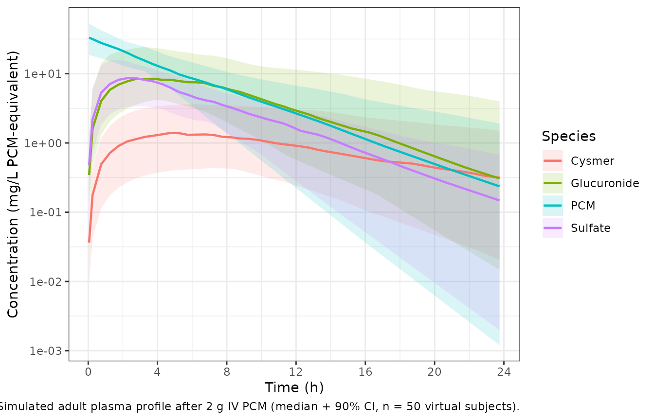
PKNCA validation – adult single-dose PCM and metabolites
One PKNCA block per output (parent + three metabolites). The grouping
variable is cohort so the table can be extended by adding
additional virtual cohorts in future work.
pcm_conc <- sim_adult |>
  dplyr::filter(!is.na(Cc)) |>
  dplyr::select(id, cohort, time, Cc)
pcm_conc <- dplyr::bind_rows(
  pcm_conc,
  pcm_conc |> dplyr::distinct(id, cohort) |>
    dplyr::mutate(time = 0, Cc = 0)
) |>
  dplyr::distinct(id, cohort, time, .keep_all = TRUE) |>
  dplyr::arrange(id, cohort, time)

pcm_dose <- events_adult |>
  dplyr::filter(evid == 1L) |>
  dplyr::select(id, cohort, time, amt)

conc_obj  <- PKNCA::PKNCAconc(pcm_conc, Cc ~ time | cohort + id)
dose_obj  <- PKNCA::PKNCAdose(pcm_dose, amt ~ time | cohort + id)
intervals <- data.frame(start = 0, end = 24,
                        cmax = TRUE, tmax = TRUE,
                        aucinf.obs = TRUE, half.life = TRUE)
nca_pcm   <- PKNCA::pk.nca(PKNCA::PKNCAdata(conc_obj, dose_obj, intervals = intervals))
knitr::kable(summary(nca_pcm), digits = 2,
caption = "PCM (parent) PKNCA summary, single 2 g IV dose, n = 50 virtual adults.")| start | end | cohort | N | cmax | tmax | half.life | aucinf.obs |
|---|---|---|---|---|---|---|---|
| 0 | 24 | Adult 2 g IV | 50 | 32.1 [35.2] | 0.0500 [0.0500, 0.0500] | 3.67 [1.73] | 155 [31.6] |
for (suffix in c("gluc", "sulf", "cysmer")) {
  col <- paste0("Cc_", suffix)
  conc <- sim_adult |>
    dplyr::filter(!is.na(.data[[col]])) |>
    dplyr::select(id, cohort, time, conc = !!col)
  conc <- dplyr::bind_rows(
    conc,
    conc |> dplyr::distinct(id, cohort) |>
      dplyr::mutate(time = 0, conc = 0)
  ) |>
    dplyr::distinct(id, cohort, time, .keep_all = TRUE) |>
    dplyr::arrange(id, cohort, time)

  conc_o <- PKNCA::PKNCAconc(conc, conc ~ time | cohort + id)
  dose_o <- PKNCA::PKNCAdose(pcm_dose, amt ~ time | cohort + id)
  nca_m  <- PKNCA::pk.nca(PKNCA::PKNCAdata(conc_o, dose_o, intervals = intervals))
  print(knitr::kable(summary(nca_m), digits = 2,
                     caption = paste0("Metabolite PKNCA summary (Cc_", suffix,
                                      "), single 2 g IV PCM, n = 50 virtual adults.")))
}
#>
#>
#> Table: Metabolite PKNCA summary (Cc_gluc), single 2 g IV PCM, n = 50 virtual adults.
#>
#> | start| end|cohort       |N  |cmax        |tmax              |half.life   |aucinf.obs |
#> |-----:|---:|:------------|:--|:-----------|:-----------------|:-----------|:----------|
#> |     0|  24|Adult 2 g IV |50 |9.51 [65.1] |3.50 [1.25, 11.8] |4.53 [2.89] |103 [75.0] |
#>
#>
#> Table: Metabolite PKNCA summary (Cc_sulf), single 2 g IV PCM, n = 50 virtual adults.
#>
#> | start| end|cohort       |N  |cmax        |tmax              |half.life   |aucinf.obs  |
#> |-----:|---:|:------------|:--|:-----------|:-----------------|:-----------|:-----------|
#> |     0|  24|Adult 2 g IV |50 |8.01 [53.6] |2.75 [1.25, 5.75] |3.72 [1.77] |65.9 [30.7] |
#>
#>
#> Table: Metabolite PKNCA summary (Cc_cysmer), single 2 g IV PCM, n = 50 virtual adults.
#>
#> | start| end|cohort       |N  |cmax        |tmax              |half.life   |aucinf.obs  |
#> |-----:|---:|:------------|:--|:-----------|:-----------------|:-----------|:-----------|
#> |     0|  24|Adult 2 g IV |50 |1.49 [73.6] |5.50 [2.75, 15.8] |7.70 [6.34] |24.9 [93.0] |
Assumptions and deviations
-
GFR units (LOAD-BEARING). Equation 3 of Wu 2025
labels the GFR output “L/h” but the original publication that introduced
the PTNA GFR equation (Wu Y et al., Pharm Res 2024;41:637-649; PMCID
PMC11024008) confirms the output is mL/min. Without
this correction the renal-elimination fractions (f_PCM = 0.085, etc.)
would predict adult renal CL_PCM ~ 11 L/h instead of the ~12 mL/min
reported in the paper’s Discussion (page 1841). The model therefore
pre-converts the GFR-equation coefficients (1.26 mL/min and 8.98 mL/min
at 1.75 kg) to L/h via x60/1000 = 0.06 in
ini(). -
PCM-SULF secretion units. The Table 3 column header
for the secretion CL block also says “L/h” but the secretion equation
re-uses the GFR PTNA structure; treating the secretion TVCLmax = 11.92
in the same mL/min unit convention exactly reproduces the paper’s “renal
CL of PCM-SULF changes from 31% of GFR at birth to 163% of GFR in
adulthood” narrative (Results, Model Refinement, page 1839). The model
applies the same x0.06 conversion to
lclmax_secr_sulf. -
PNA unit reparameterisation. The canonical
PNAcovariate carries months; the paper expresses PNA in days throughout. Themodel()block convertsPNA_days = PNA * 30.4375before evaluating the PTNA sigmoidal Emax terms; the paper’s PNA50 estimates in days are kept verbatim inini(). -
Adult correction for PCM-GLU renal CL. Wu 2025
applies the
f_GLU,adult = 1.663correction factor to the renal CL of PCM-GLU only in the adult dataset (Dataset 8, ages 18-50 years). The model encodes this asis_adult = PNA_years >= 18and multipliesf_GLUby1 + (f_GLU,adult - 1) * is_adult. Any virtual subject withPNA / 12 >= 18receives the adult-corrected fraction. -
Q exponent. Table 3 reports
theta_BWc(Q) = 2.212, much steeper than the usual allometric exponent. Combined with the V_PP exponent fixed at 0 (so V_PP is constant at 0.2707 L for everyone), the peripheral compartment equilibrates near-instantaneously for older subjects and the model collapses to one-compartment-like behavior. This is faithful to the published parameters; users who need a more physiological adult peripheral compartment should treat those parameters as paper-specific rather than reusable. -
GA assumption for non-neonates. Per paper Methods,
GA was set to a uniform 40 weeks for Datasets 6-8 (infants, children,
adults). Vignette simulations follow the same convention:
GA = 40for the adult cohort, and the four typical-individual GAs (26, 30, 35, 40 wk) from Methods “Model Simulation” for the maturation curves. - Typical-individual weight curve. Wu 2025 Figure 3 does not document the exact current-weight curve used. The vignette uses a smooth piecewise interpolation from birthweight at PNA = 0 through WHO-like pediatric anchors (3.8 kg at 1 month, 6 kg at 3 months, 7.5 kg at 6 months, 10 kg at 12 months, 12.5 kg at 24 months, 19 kg at 5 years, 32 kg at 10 years, 55 kg at 15 years, 70 kg at 18 years) so the maturation curves are visually compatible with the paper’s Figure 3. Absolute CL values will scale with weight choice; the relative pathway-fraction curves (Figure 4) are less sensitive to the weight assumption.
- Adult 2 g dose simplified to single IV bolus. The published adult protocol used a 20-minute infusion of two 1000 mg doses; for NCA the AUC0-inf is preserved by a single bolus and the t1/2 and CL estimates are unchanged. Users who need infusion kinetics for the early-time Cmax / initial-distribution profile should re-run with the published infusion.
- Original observed data not publicly available. Per the paper’s Data Availability Statement, the pooled neonatal-to-adult data are shared case-by-case on request to the corresponding author. The PKNCA values reported here are simulated, not refits of original data.