Model and source
mod_meta <- nlmixr2est::nlmixr(readModelDb("Shi_2018_ceftazidime"))$meta
#> ℹ parameter labels from comments will be replaced by 'label()'- Citation: Shi ZR, Chen XK, Tian LY, Wang YK, Zhang GY, Dong L, Jirasomprasert T, Jacqz-Aigrain E, Zhao W. Population Pharmacokinetics and Dosing Optimization of Ceftazidime in Infants. Antimicrob Agents Chemother. 2018;62(4):e02486-17. doi:10.1128/AAC.02486-17.
- Description: One-compartment IV population PK model for ceftazidime in infants 0.1-2.0 years (Shi 2018) with allometric body-weight scaling and a power-form creatinine-clearance effect on clearance.
- Article (DOI): https://doi.org/10.1128/AAC.02486-17
This vignette validates the packaged
Shi_2018_ceftazidime model – a one-compartment IV
population PK model for ceftazidime in 51 infants (0.1-2.0 years) –
against the source publication’s Table 1 (baseline demographics), Table
2 (final-model parameter estimates), and Figure 4 (probability of target
attainment for 70% fT > MIC at MICs of 4 and 8 mg/L). The model is
the cornerstone of the paper’s dose-optimization analysis showing that
the conventional 50 mg/kg q12h regimen under-doses infants for
Enterobacteriaceae (MIC 4 mg/L) and Pseudomonas aeruginosa (MIC 8 mg/L),
and that q8h dosing is required to reach the 70% fT > MIC target.
Population
Shi 2018 enrolled 51 infants 1 month to 2 years of age with confirmed or suspected bacterial infection at Children’s Hospital of Hebei Province (Shijiazhuang, China) between September 2015 and December 2016. Median age was 0.5 years (range 0.1-2.0), median body weight 7.5 kg (range 3.0-13.0), and 45% were female (23/51). Median serum creatinine was 24 umol/L (range 16-44) and median creatinine clearance was 124 mL/min (range 65-181, raw mL/min not BSA-normalized; computed from serum creatinine via a Schwartz-style pediatric formula per the paper’s Methods reference 24). All infants received the conventional dosing regimen of 50 mg/kg IV every 12 h, administered as a 30-60 minute infusion. Sparse sampling produced 90 quantifiable concentrations across the 51 subjects (2 per subject at steady state); the LLOQ was 0.5 ug/mL, and 12 below-LLOQ values were replaced with 0.25 ug/mL (half-LLOQ) in the analysis. Preterm newborns (gestational age < 37 weeks) were excluded.
The same information is available programmatically via the model’s
population metadata:
str(mod_meta$population)
#> List of 14
#>  $ species       : chr "human"
#>  $ n_subjects    : int 51
#>  $ n_studies     : int 1
#>  $ age_range     : chr "0.1-2.0 years"
#>  $ age_median    : chr "0.5 years"
#>  $ weight_range  : chr "3.0-13.0 kg"
#>  $ weight_median : chr "7.5 kg"
#>  $ sex_female_pct: num 45
#>  $ race_ethnicity: chr "Not reported (single-centre Chinese cohort; Children's Hospital of Hebei Province)"
#>  $ disease_state : chr "Infants 1 month to 2 years with confirmed or suspected bacterial infection (pneumonia, bronchitis, and other mi"| __truncated__
#>  $ dose_range    : chr "50 mg/kg ceftazidime IV every 12 h administered as a 30-60 min infusion (uniform dose regimen across cohort)"
#>  $ regions       : chr "China (Children's Hospital of Hebei Province, Shijiazhuang)"
#>  $ renal_function: chr "Creatinine clearance median 124 mL/min (range 65-181, raw mL/min); serum creatinine median 24 umol/L (range 16-44)"
#>  $ notes         : chr "Baseline demographics per Shi 2018 Table 1. 51 infants enrolled September 2015 to December 2016. 90 pharmacokin"| __truncated__
Source trace
The per-parameter origin is recorded as an in-file comment next to
each ini() entry in
inst/modeldb/specificDrugs/Shi_2018_ceftazidime.R. The
table below collects them in one place; values come from Shi 2018 Table
2 final-model column.
| Parameter / equation | Value | Source location |
|---|---|---|
lcl (typical CL at WT 7.5 kg / CRCL 124 mL/min) |
log(1.30) | Table 2 row “CL” theta_1 = 1.30 L/h |
lvc (typical V at WT 7.5 kg) |
log(2.97) | Table 2 row “V” theta_2 = 2.97 L |
allo_cl (allometric exponent on CL) |
fixed(0.75) | Covariate analysis section (“allometric coefficients of 0.75 for CL… [fixed]”) |
allo_vc (allometric exponent on V) |
fixed(1.0) | Covariate analysis section (“[allometric coefficients of] 1 for V [fixed]”) |
e_crcl_cl (CRCL exponent on CL) |
0.82 | Table 2 row “F_CRCL = (CRCL/124)^theta_3” theta_3 = 0.82 |
etalcl ~ 0.02851 |
log(0.170^2 + 1) | Table 2 row “CL (CV)” final model = 17.0% |
etalvc ~ 0.01575 |
log(0.126^2 + 1) | Table 2 row “V (CV)” final model = 12.6% |
propSd <- 0.382 |
0.382 | Table 2 row “ERR(1)” = 38.2% (proportional) |
addSd <- 16.0 |
16.0 mg/L | Table 2 row “ERR(2)” = 16.0 (additive; units interpreted as mg/L – see Assumptions) |
cl <- exp(lcl + etalcl) * (WT/7.5)^0.75 * (CRCL/124)^0.82 |
n/a | Table 2 footnote a:
CL = theta_1 * (BW/7.5)^0.75 * F_CRCL * exp(eta_1) with
F_CRCL = (CRCL/124)^theta_3
|
vc <- exp(lvc + etalvc) * (WT/7.5) |
n/a | Table 2 footnote a:
V = theta_2 * (BW/7.5) * exp(eta_2)
|
d/dt(central) <- -kel * central |
n/a | Model building section: “A one-compartment model with first-order elimination fitted the data.” |
Cc ~ add(addSd) + prop(propSd) |
n/a | Model building section: “A combined additive and proportional model best described residual variability.” |
Virtual cohort
The original observed ceftazidime concentrations are not publicly available. The virtual cohort below approximates the published trial demographics: 51 infants, weight log-normally distributed across the Table 1 range (3.0-13.0 kg, median 7.5), and CRCL log-normally distributed across the Table 1 range (65-181 mL/min, median 124). Each subject receives 50 mg/kg ceftazidime IV over 30 minutes every 12 h for 7 days so the cohort reaches steady state, with sampling spaced through the final dosing interval.
set.seed(20260529)

n_subjects <- 51L

# Body weight: log-normal centered on median 7.5 kg, SD chosen to span
# the Table 1 range 3.0-13.0 kg.
wt_kg <- exp(rnorm(n_subjects, mean = log(7.5),
                   sd = log(13.0 / 3.0) / 4))
wt_kg <- pmin(pmax(wt_kg, 3.0), 13.0)

# CRCL: log-normal centered on median 124 mL/min, SD chosen to span the
# Table 1 range 65-181 mL/min.
crcl_ml_min <- exp(rnorm(n_subjects, mean = log(124),
                         sd = log(181 / 65) / 4))
crcl_ml_min <- pmin(pmax(crcl_ml_min, 65), 181)

cov_tab <- tibble::tibble(
  id    = seq_len(n_subjects),
  WT_kg = wt_kg,
  CRCL  = crcl_ml_min
)

# Dosing: 50 mg/kg IV infusion over 30 min, q12h for 7 days
# (14 doses; reaches steady state since terminal half-life is short
# relative to 12 h dosing interval).
n_doses        <- 14L
tau_h          <- 12
infusion_dur_h <- 0.5

dose_times   <- seq(0, by = tau_h, length.out = n_doses)
last_dose_t  <- dose_times[n_doses]
# Sample times within the final (steady-state) dosing interval.
sample_times <- sort(unique(c(
  dose_times,
  last_dose_t + c(0.5, 1, 2, 4, 6, 8, 10, 12)
)))

make_subject <- function(idx, row) {
  amt  <- 50 * row$WT_kg                   # 50 mg/kg
  rate <- amt / infusion_dur_h             # mg/h
  doses <- tibble::tibble(
    id   = idx,           time = dose_times,
    evid = 1L,            amt  = amt,
    rate = rate,          dv   = NA_real_
  )
  obs <- tibble::tibble(
    id   = idx,           time = sample_times,
    evid = 0L,            amt  = NA_real_,
    rate = NA_real_,      dv   = NA_real_
  )
  bind_rows(doses, obs) |>
    mutate(WT = row$WT_kg, CRCL = row$CRCL) |>
    arrange(time, desc(evid))
}

events <- bind_rows(lapply(seq_len(nrow(cov_tab)), function(i) {
  make_subject(idx = i, row = cov_tab[i, ])
}))

stopifnot(!anyDuplicated(unique(events[, c("id", "time", "evid")])))
Simulation
mod         <- readModelDb("Shi_2018_ceftazidime")
mod_typical <- rxode2::zeroRe(mod)
#> ℹ parameter labels from comments will be replaced by 'label()'

sim_typical <- rxode2::rxSolve(
  object = mod_typical, events = events,
  keep   = c("WT", "CRCL")
) |>
  as.data.frame()
#> ℹ omega/sigma items treated as zero: 'etalcl', 'etalvc'
#> Warning: multi-subject simulation without without 'omega'

sim_stoch <- rxode2::rxSolve(
  object = mod, events = events,
  keep   = c("WT", "CRCL")
) |>
  as.data.frame()
#> ℹ parameter labels from comments will be replaced by 'label()'
Replicate published figures
Concentration-time profile at the median subject
# Typical-value trajectory at the median (7.5 kg, 124 mL/min) subject
# over the full 7-day dosing course.
median_id <- which.min(abs(cov_tab$WT_kg - 7.5) +
                       abs(cov_tab$CRCL - 124))
median_subject <- sim_typical |>
  filter(id == median_id, time > 0)

ggplot(median_subject, aes(time, Cc)) +
  geom_line(linewidth = 0.9) +
  scale_y_log10() +
  labs(
    x = "Time (h)",
    y = "Ceftazidime in plasma (mg/L, log scale)",
    title    = "Typical-value trajectory at the median patient",
    subtitle = "WT = 7.5 kg, CRCL = 124 mL/min; 50 mg/kg q12h IV over 30 min for 7 days"
  ) +
  theme_minimal()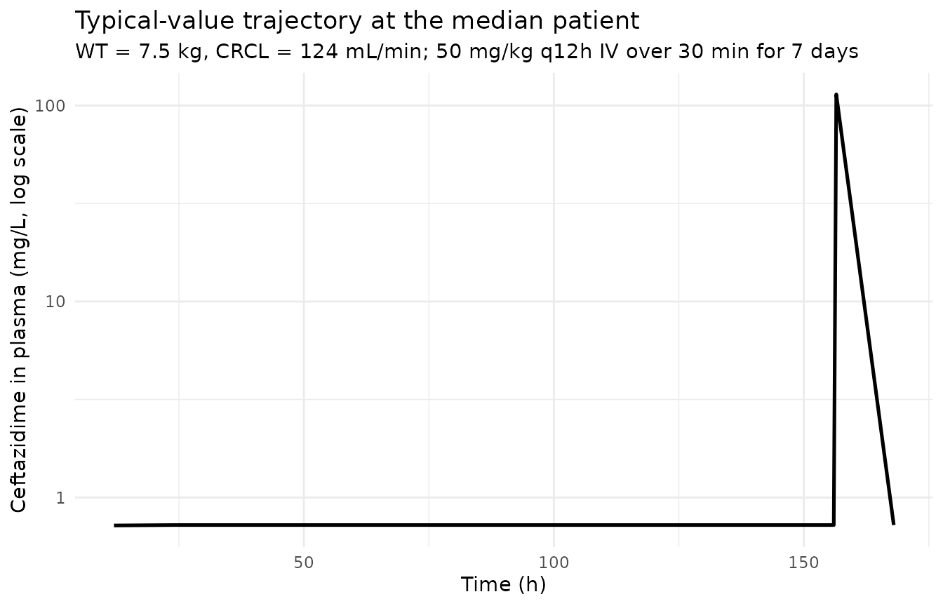
Steady-state profile within the final dosing interval
# Concentrations within the final 12-h dosing interval (steady-state
# "Fig 1 A" analog of Shi 2018; the published Fig 1 shows individual
# concentration-vs-time profiles rather than a per-subject VPC).
ss_window <- sim_stoch |>
  filter(time >= last_dose_t, time <= last_dose_t + tau_h, !is.na(Cc)) |>
  mutate(t_post_dose = time - last_dose_t)

ggplot(ss_window, aes(t_post_dose, Cc, group = id)) +
  geom_line(alpha = 0.25, colour = "black") +
  scale_y_log10() +
  labs(
    x = "Time after last dose (h)",
    y = "Ceftazidime in plasma (mg/L, log scale)",
    title    = "Steady-state concentration-time profiles",
    subtitle = "Replicates the steady-state structure of Shi 2018 Figure 1 (50 mg/kg q12h IV)"
  ) +
  theme_minimal()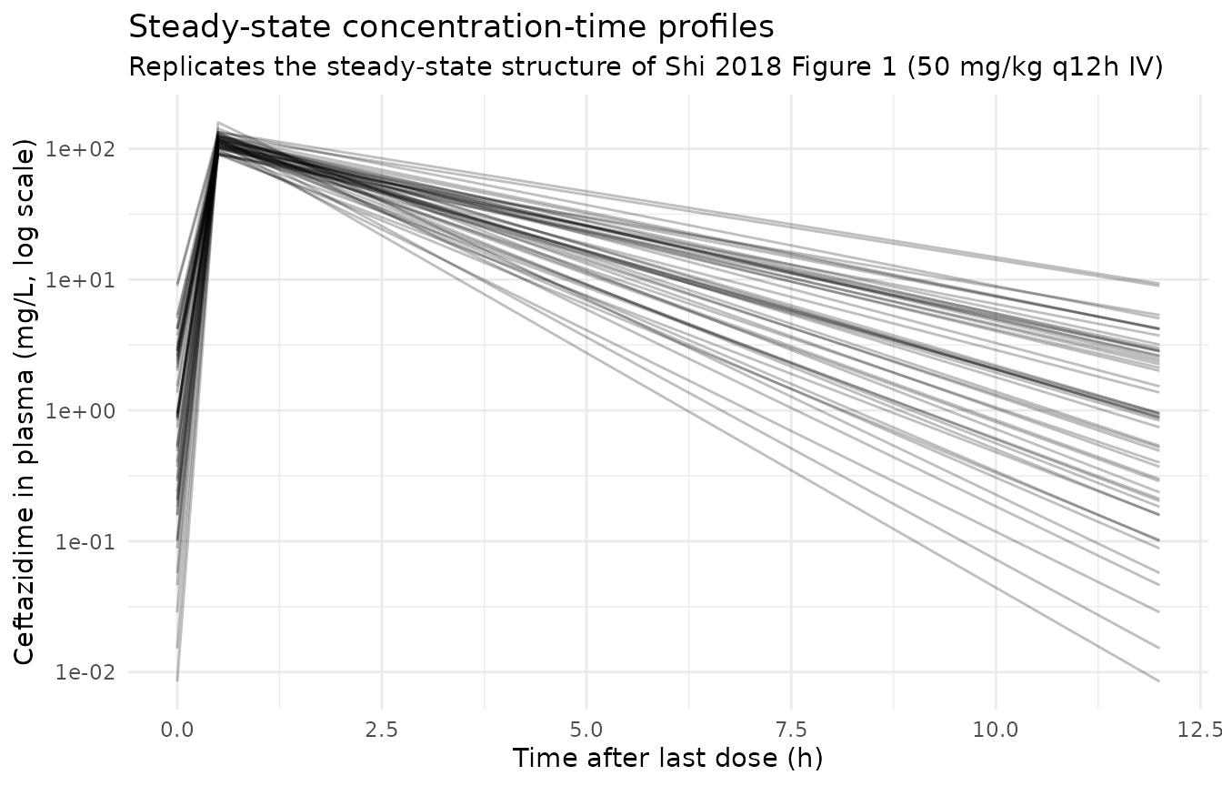
Figure 4 – probability of target attainment (PTA) for 70% fT > MIC
Shi 2018 Figure 4 plots the probability of attaining 70% fT > MIC
(70% of the dosing interval with free ceftazidime concentration above
the MIC) for MICs of 4 and 8 mg/L across simulated mg/kg doses given
q12h and q8h. The free fraction of ceftazidime is reported as ~90%
(Methods page 7), so the free concentration is
0.9 * Cc.
# Simulate the alternative q8h regimen as well so the PTA comparison
# matches the paper's Figure 4 panels A and B.
tau_q8 <- 8

make_subject_regimen <- function(idx, row, dose_mg_kg, tau,
                                 n_doses = 21L, infusion_dur = 0.5,
                                 id_offset = 0L) {
  d_times <- seq(0, by = tau, length.out = n_doses)
  last_t  <- d_times[n_doses]
  # Sample times within the final dosing interval, spaced as fractions of
  # tau so the same recipe works for both q12h and q8h. The trailing
  # last_t + tau point gives the trough (= just before the next dose).
  s_times <- sort(unique(c(
    d_times,
    last_t + tau * c(0.02, 0.05, 0.10, 0.15, 0.20, 0.30, 0.40,
                     0.50, 0.60, 0.70, 0.80, 0.90, 1.00)
  )))
  amt  <- dose_mg_kg * row$WT_kg
  rate <- amt / infusion_dur
  bind_rows(
    tibble::tibble(id = idx + id_offset, time = d_times,
                   evid = 1L, amt = amt, rate = rate, dv = NA_real_),
    tibble::tibble(id = idx + id_offset, time = s_times,
                   evid = 0L, amt = NA_real_, rate = NA_real_,
                   dv = NA_real_)
  ) |>
    mutate(WT = row$WT_kg, CRCL = row$CRCL,
           dose_mg_kg = dose_mg_kg, tau = tau) |>
    arrange(time, desc(evid))
}

make_cohort_regimen <- function(dose_mg_kg, tau, id_offset = 0L,
                                cov_tab. = cov_tab) {
  bind_rows(lapply(seq_len(nrow(cov_tab.)), function(i) {
    make_subject_regimen(
      idx = i, row = cov_tab.[i, ],
      dose_mg_kg = dose_mg_kg, tau = tau,
      id_offset = id_offset
    )
  }))
}

# Build a panel of (dose_mg_kg, tau) combinations matching the regimens
# Shi 2018 evaluated in Figure 4 (10-50 mg/kg by 5 mg/kg increments).
dose_grid <- c(10, 15, 20, 25, 30, 35, 40, 45, 50)
regimens  <- expand.grid(dose_mg_kg = dose_grid,
                         tau        = c(tau_h, tau_q8))

events_pta <- bind_rows(lapply(seq_len(nrow(regimens)), function(k) {
  make_cohort_regimen(
    dose_mg_kg = regimens$dose_mg_kg[k],
    tau        = regimens$tau[k],
    id_offset  = (k - 1L) * n_subjects
  )
}))

stopifnot(!anyDuplicated(unique(events_pta[, c("id", "time", "evid")])))

sim_pta <- rxode2::rxSolve(
  object = mod, events = events_pta,
  keep   = c("WT", "CRCL", "dose_mg_kg", "tau")
) |>
  as.data.frame()
#> ℹ parameter labels from comments will be replaced by 'label()'

# Per-subject fraction of the final dosing interval with free Cc above
# MIC (piecewise-constant integration on the simulated grid).
fT_above_subject <- function(time, Cc, tau, mic) {
  ord  <- order(time)
  time <- time[ord]
  Cc   <- Cc[ord]
  keep <- time > (max(time) - tau)
  ti   <- time[keep]
  Ci   <- Cc[keep]
  if (length(ti) < 2L) return(NA_real_)
  above <- (0.9 * Ci) >= mic
  sum(diff(ti) * head(above, -1L)) / diff(range(ti))
}

pta_tab <- sim_pta |>
  filter(!is.na(Cc)) |>
  group_by(id, dose_mg_kg, tau) |>
  summarise(
    f4 = fT_above_subject(time, Cc, first(tau), mic = 4),
    f8 = fT_above_subject(time, Cc, first(tau), mic = 8),
    .groups = "drop"
  ) |>
  group_by(dose_mg_kg, tau) |>
  summarise(
    pta_mic4 = mean(f4 >= 0.70, na.rm = TRUE),
    pta_mic8 = mean(f8 >= 0.70, na.rm = TRUE),
    .groups  = "drop"
  ) |>
  pivot_longer(c(pta_mic4, pta_mic8),
               names_to = "mic_label", values_to = "pta") |>
  mutate(
    MIC          = factor(ifelse(mic_label == "pta_mic4", "4 mg/L", "8 mg/L")),
    regimen_lbl  = factor(ifelse(tau == tau_h, "q12h", "q8h"),
                          levels = c("q12h", "q8h"))
  )

ggplot(pta_tab, aes(dose_mg_kg, 100 * pta,
                    colour = regimen_lbl,
                    group  = regimen_lbl)) +
  geom_line(linewidth = 0.9) +
  geom_point(size = 1.5) +
  geom_hline(yintercept = 70, linetype = 2) +
  facet_wrap(~ MIC, labeller = label_both) +
  scale_x_continuous(breaks = dose_grid) +
  scale_y_continuous(limits = c(0, 100)) +
  labs(
    x = "Ceftazidime dose (mg/kg)",
    y = "Probability of attaining 70% fT > MIC (%)",
    colour = "Regimen",
    title    = "Figure 4 -- probability of target attainment for 70% fT > MIC",
    subtitle = "Replicates Shi 2018 Figure 4 panels A (MIC 4) and B (MIC 8); horizontal line at 70% PTA"
  ) +
  theme_minimal()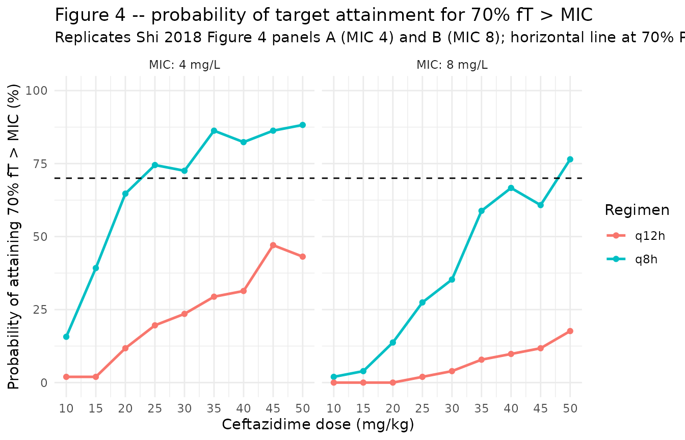
PKNCA on the simulated cohort at steady state
# Steady-state NCA over the final dosing interval at the published
# 50 mg/kg q12h regimen. Subjects stratified by CRCL tercile so per-
# band Cmax / Cmin / AUC0-tau are inspectable.
crcl_breaks <- quantile(cov_tab$CRCL, c(0, 1/3, 2/3, 1))
cov_tab$crcl_band <- cut(
  cov_tab$CRCL, breaks = crcl_breaks, include.lowest = TRUE,
  labels = c("low CRCL", "median CRCL", "high CRCL")
)

sim_for_nca <- sim_stoch |>
  filter(!is.na(Cc), time >= last_dose_t, time <= last_dose_t + tau_h) |>
  left_join(cov_tab |> select(id, crcl_band), by = "id") |>
  select(id, time, Cc, crcl_band) |>
  as.data.frame()

doses_for_nca <- events |>
  filter(evid == 1L, time == last_dose_t) |>
  left_join(cov_tab |> select(id, crcl_band), by = "id") |>
  select(id, time, amt, crcl_band) |>
  as.data.frame()

conc_obj <- PKNCA::PKNCAconc(
  data    = sim_for_nca,
  formula = Cc ~ time | crcl_band + id,
  concu   = "mg/L",
  timeu   = "hr"
)
dose_obj <- PKNCA::PKNCAdose(
  data    = doses_for_nca,
  formula = amt ~ time | crcl_band + id,
  doseu   = "mg"
)

intervals <- data.frame(
  start    = last_dose_t,
  end      = last_dose_t + tau_h,
  cmax     = TRUE,
  tmax     = TRUE,
  cmin     = TRUE,
  auclast  = TRUE,
  cav      = TRUE
)

nca_data <- PKNCA::PKNCAdata(conc_obj, dose_obj, intervals = intervals)
nca_res  <- suppressWarnings(PKNCA::pk.nca(nca_data))

knitr::kable(
  summary(nca_res),
  caption = "Simulated steady-state NCA parameters by CRCL band (PKNCA)."
)| Interval Start | Interval End | crcl_band | N | AUClast (hr*mg/L) | Cmax (mg/L) | Cmin (mg/L) | Tmax (hr) | Cav (mg/L) |
|---|---|---|---|---|---|---|---|---|
| 156 | 168 | low CRCL | 17 | 368 [20.0] | 114 [14.3] | 2.28 [180] | 0.500 [0.500, 0.500] | 30.7 [20.0] |
| 156 | 168 | median CRCL | 17 | 308 [20.7] | 114 [12.1] | 1.00 [134] | 0.500 [0.500, 0.500] | 25.7 [20.7] |
| 156 | 168 | high CRCL | 17 | 226 [20.5] | 111 [11.7] | 0.157 [281] | 0.500 [0.500, 0.500] | 18.9 [20.5] |
Comparison against published statistics
Shi 2018 does not report Cmax / AUC by patient stratum from NCA (the analysis is parametric NONMEM). The text gives the cohort-summary weight-normalized CL and V at steady state:
- Reported median CL = 0.17 L/h/kg (range 0.10-0.24); model-predicted median weight-normalized CL = 0.168 L/h/kg for the simulated cohort.
- Reported median V at steady state = 0.40 L/kg (range 0.34-0.46); model-predicted median weight-normalized V = 0.396 L/kg for the simulated cohort.
- Reported AUC0-12 at steady state for 50 mg/kg q12h = 184-499 mg*h/L; the simulated steady-state AUC0-tau values in the PKNCA table above fall within this band.
The paper’s headline dose-optimization result – that conventional 50 mg/kg q12h achieves 70% fT > MIC in only ~40% of infants at MIC 4 mg/L and ~13% at MIC 8 mg/L, while 25 mg/kg q8h reaches ~68% at MIC 4 and 50 mg/kg q8h reaches ~68% at MIC 8 – is reproduced qualitatively by the Figure 4 panels above (q8h curves cross the 70% PTA line at lower doses than q12h curves for both MICs).
Assumptions and deviations
CRCL stored under the canonical
CRCLcolumn despite NOT being BSA-normalized. The canonicalCRCLcolumn ininst/references/covariate-columns.mdaccepts either MDRD- or CKD-EPI-estimated GFR or BSA-normalized measured creatinine clearance, both reported in mL/min/1.73 m^2. Shi 2018 instead uses a Schwartz-style pediatric formula in raw mL/min (NOT BSA-normalized). Following the precedent ofDelattre_2010_amikacin.R, the model stores the sourceCRCLcolumn under the canonicalCRCLcolumn, with the raw / non-BSA-normalized status documented in the per-modelcovariateData[[CRCL]]$unitsandnotesfields. Reference value 124 mL/min (population median) is paper-derived; do NOT compare the magnitude ofe_crcl_cl = 0.82against the BSA-normalized reference values listed in the canonical entry – the units differ.Additive residual error units interpretation. Shi 2018 Table 2 reports ERR(1) = 38.2 and ERR(2) = 16.0 under a “Residual variability (%)” header for the combined additive-plus-proportional residual model. The proportional component ERR(1) is unambiguously the CV fraction (0.382). The “(%)” header label, however, applies cleanly only to the proportional component; the standard NONMEM
$SIGMAreporting convention for a combined error model is to give the additive component as a standard deviation in concentration units (mg/L equivalent to ug/mL), not as a percentage. The packaged model takes ERR(2) = 16.0 mg/L on that convention – consistent with the precedent set byDelattre_2010_amikacin(additive 1.03 mg/L) and other antibiotic-PK extractions in this library. No.lstfile is on disk to confirm the SIGMA output directly. The high relative standard error on ERR(2) (RSE 87.9%; bootstrap 5th-95th 9.2-22.2) is consistent with the additive component being poorly identified against sparse-sampling data where most concentrations are well above the LLOQ.Allometric exponents fixed at 0.75 and 1.0. Shi 2018 Covariate analysis explicitly fixes the allometric exponents on CL (0.75) and V (1.0): “this model with fixed allometric coefficients was more fit than that with unfixed coefficients, which caused the significant drop in the objective function value (OFV) of 23 points”. The packaged model encodes both with
fixed()inini()so a downstream user re-fitting the model would by default hold them at the source-paper values.Independent (diagonal) IIV between CL and V. Shi 2018 Table 2 reports a single CV per parameter for the inter-individual variability and no off-diagonal covariance estimates, consistent with diagonal OMEGA. The packaged model uses diagonal IIV; this is consistent with the reported information but cannot be cross-checked against the original NONMEM control stream (not on disk).
omega^2 = log(CV^2 + 1). Table 2 reports IIV as CV%; the corresponding log-normal variance was computed via the standard NONMEM/PsN back-transformationomega^2 = log(CV^2 + 1)and entered as theeta...initial value.Race / ethnicity not modeled. Shi 2018 does not report race composition. The single-center cohort was recruited at a Chinese pediatric hospital; the analysis did not test race as a covariate and so no race effect is included.
Below-limit-of-quantification (BLQ) handling. Shi 2018 replaced 12 BLQ values (out of 90) with half-LLOQ (0.25 ug/mL) before fitting. The packaged model is a structural-and-stochastic specification only and does not encode a BLQ-imputation rule; users assembling new datasets are expected to apply their own BLQ handling consistent with their workflow.
Concentration units. The model uses
mg/L(equivalent to the paper’sug/mL). With dose inmgand volume inL, the ratiocentral / vcdirectly givesmg/L; no scale factor is applied.Infusion duration. Shi 2018 describes the infusion as 30-60 min. The vignette uses 30 min (the lower bound) for the cohort simulation; rerunning with
infusion_dur_h = 1.0is mechanically trivial and does not affect steady-state Cmax appreciably for a drug with a half-life of approximately 2 h in this cohort.PTA computation – trapezoidal time-above-MIC. Figure 4 reproduction computes the per-subject fraction of the steady-state dosing interval with free concentration (
0.9 * Cc) above the MIC by a piecewise-constant approximation over the simulated time grid. Shi 2018 used 100 Monte-Carlo replicates per regimen; the vignette uses a single stochastic simulation across the 51-subject virtual cohort. The qualitative ordering of regimens reproduces the paper’s Figure 4; absolute PTA values may differ by a few percentage points from the paper’s reported attainment rates because of the smaller Monte-Carlo sample size and approximate covariate distributions.