Model and source
- Citation: Jiao Z, Shi XJ, Li ZD, Zhong MK. Population pharmacokinetics of sirolimus in de novo Chinese adult renal transplant patients. Br J Clin Pharmacol. 2009;68(1):47-54. doi:10.1111/j.1365-2125.2009.03392.x.
- Description: One-compartment population PK model for oral sirolimus in Chinese adult de novo renal transplant recipients on triple immunosuppression with ciclosporin and corticosteroids (Jiao 2009). First-order absorption with ka fixed at the literature value 0.752 1/h. Covariate effects on apparent clearance: linear-deviation effects of total cholesterol and whole-blood ciclosporin trough concentration centred on the cohort medians, multiplicative power-form effects of concomitant silymarin and glycyrrhizin co-therapy in hepatically impaired patients, and a power-form effect of the current sirolimus daily dose centred at 2 mg. Apparent volume of distribution carries a linear-deviation effect of ciclosporin trough concentration.
- Article: https://doi.org/10.1111/j.1365-2125.2009.03392.x
Jiao, Shi, Li, and Zhong (Huashan Hospital, Fudan University) developed a one-compartment population PK model for oral sirolimus from 804 trough concentrations collected in 112 Chinese adult de novo renal transplant recipients enrolled at five clinical centres (Methods + Results). All patients received induction therapy with ciclosporin (CsA), sirolimus, and corticosteroids during the first three months, followed by either CsA dose reduction (Phase I) or CsA discontinuation (Phase II). Because the sampling design was trough-only, the absorption rate ka was held at the literature value 0.752 1/h (Zahir et al. 2006, paper ref [32]) and apparent clearance (CL/F) and apparent volume of distribution (V/F) were the estimated parameters. After forward stepwise inclusion and backward elimination, five covariates were retained on CL/F (total cholesterol, CsA trough concentration, sirolimus daily dose, silymarin co-therapy, glycyrrhizin co-therapy) and one on V/F (CsA trough concentration). The model is the first population PK characterisation of sirolimus in Chinese renal transplant patients and is notable for identifying silymarin (milk thistle) and glycyrrhizin (licorice) co-therapy as novel covariates on sirolimus CL/F in hepatically impaired patients.
Population
The model-development cohort comprised 112 Chinese adult de novo primary renal allograft recipients (78 male / 34 female; 30.4 percent female) enrolled across five clinical centres in Guangzhou, Shanghai, and Beijing between June 2004 and August 2006 (Methods, Study design; Table 1). Mean age was 42 years (range 19-68), mean body weight 60.4 kg (range 44.5-91.0), mean body surface area 1.70 m^2 (range 1.33-2.18). The cohort split between Phase I (n = 71, CsA dose reduction) and Phase II (n = 41, CsA discontinuation), with most allografts sourced from cadaveric donors (104 of 112, 93 percent). Sirolimus was initiated at a loading dose of 6 mg PO within 24 h of transplant surgery, followed by a maintenance dose of 0.5-6 mg/day titrated to whole-blood trough targets (6-12 ng/mL months 1-3, 12-20 ng/mL months 4-6 of Phase II, 10-20 ng/mL months 7-12 of Phase II). The trial is registered as NCT00257387 and was sponsored by Wyeth Pharmaceutical Co., Ltd., China.
Bioanalysis used three external laboratories with two HPLC-UV methods and one LC-MS/MS method, with all three validated through the International Sirolimus Proficiency Testing Scheme. CsA whole-blood concentrations were measured by automated fluorescence polarisation with monoclonal antibodies (AxSYM at Shanghai sites, TDx at the other three sites); no assay cross-normalisation was applied to the original C0 values in the final model (sensitivity analysis showed assay-rescaling shifted CsA-related parameters by < 20 percent with < 2 OFV units alternation).
The same information is available programmatically via the model’s
population metadata.
mod <- readModelDb("Jiao_2009_sirolimus")
str(rxode2::rxode(mod)$population)
#> ℹ parameter labels from comments will be replaced by 'label()'
#> List of 18
#>  $ species        : chr "human"
#>  $ n_subjects     : int 112
#>  $ n_observations : int 804
#>  $ n_studies      : int 1
#>  $ n_centres      : int 5
#>  $ age_range      : chr "19-68 years"
#>  $ age_median     : chr "42 years (mean 42 +/- 9.9)"
#>  $ weight_range   : chr "44.5-91.0 kg"
#>  $ weight_median  : chr "60.0 kg (mean 60.4 +/- 9.43)"
#>  $ sex_female_pct : num 30.4
#>  $ race_ethnicity : chr "Chinese (single-country multicentre cohort across Guangzhou, Shanghai and Beijing)."
#>  $ disease_state  : chr "Chinese adult de novo primary renal allograft recipients on triple immunosuppression. Patients with active majo"| __truncated__
#>  $ dose_range     : chr "Loading 6 mg PO within 24 h of transplant surgery, followed by 0.5-6.0 mg/day maintenance titrated to whole-blo"| __truncated__
#>  $ regions        : chr "China (first Affiliated Hospital of Sun Yat-Sen University, Changzheng Hospital of Second Military Medical Univ"| __truncated__
#>  $ transplant_type: chr "Primary renal allograft; cadaveric n = 104 (93%), living donor n = 8 (7%)."
#>  $ co_medication  : chr "Ciclosporin (CsA, twice daily, sirolimus dosed 4 h after morning CsA), corticosteroids (no withdrawal permitted"| __truncated__
#>  $ trial_design   : chr "Phase I (CsA dose reduction, n = 71) and Phase II (CsA discontinuation, n = 41) sub-cohorts; both arms received"| __truncated__
#>  $ notes          : chr "Eight hundred and four sirolimus trough concentrations from 112 subjects; median 6 (range 1-18) concentrations "| __truncated__
Source trace
The per-parameter origin is recorded as an in-file comment next to
each ini() entry in
inst/modeldb/specificDrugs/Jiao_2009_sirolimus.R. The table
below collects the same information in one place for review.
| Equation / parameter | Value | Source location |
|---|---|---|
lcl (typical CL/F at cohort-median covariates,
L/h) |
10.1 | Table 2 theta1 = 10.1 L/h (3.0% RSE) |
lvc (typical V/F at CsA-trough reference, L) |
3670 | Table 2 theta7 = 3670 L (9.3% RSE) |
lka (ka, 1/h; literature-fixed) |
0.752 | Methods + paper ref [32] (Zahir 2006); ka fixed, IIV not estimated |
e_tchol_cl (linear-deviation effect of TCHOL on CL/F,
L/h per mmol/L) |
-0.662 | Table 2 theta2 = 0.662 (25.1% RSE); minus sign per Eq. 9 bracket |
e_cp_csa_ngml_cl (linear-deviation effect of CsA C0 on
CL/F, L/h per ng/mL) |
-0.00417 | Table 2 theta3 = 4.17e-3 (44.4% RSE); minus sign per Eq. 9 |
e_conmed_silymarin_cl (log effect of silymarin on
CL/F) |
log(0.650) | Table 2 theta4 = 0.650 (16.3% RSE); 35% reduction in CL/F |
e_conmed_glycyrrhizin_cl (log effect of glycyrrhizin on
CL/F) |
log(0.661) | Table 2 theta5 = 0.661 (25.4% RSE); 34% reduction in CL/F |
e_dose_cl (power exponent of (DOSE/2) on CL/F) |
0.479 | Table 2 theta6 = 0.479 (16.6% RSE) |
e_cp_csa_ngml_vc (linear-deviation effect of CsA C0 on
V/F, L per ng/mL) |
-7.27 | Table 2 theta8 = 7.27 (14.9% RSE); minus sign per Eq. 10 |
etalcl (omega^2 on log CL/F) |
0.0551 | Table 2 omega_CL/F = 23.8% (26.7% RSE); omega^2 = log(1 + 0.238^2) |
etalvc (omega^2 on log V/F) |
0.2789 | Table 2 omega_V/F = 56.7% (24.8% RSE); omega^2 = log(1 + 0.567^2) |
expSd (log-normal residual SD) |
0.299 | Table 2 sigma = 29.9% (8.0% RSE); exponential error model per Methods Eq. 3 |
Final equation:
CL/F = [theta1 - theta2*(TC - 5.66) - theta3*(C0 - 104)] * theta4^SLM * theta5^GLZ * (DDS/2)^theta6
|
n/a | Eq. 9 (page 52); also reproduced in Table 2 footer |
Final equation: V/F = theta7 - theta8*(C0 - 104)
|
n/a | Eq. 10 (page 52); also reproduced in Table 2 footer |
| Cohort medians used as covariate references (TC = 5.66, C0 = 104, DDS = 2) | n/a | Table 1: TC median 5.66 mmol/L, CsA C0 median 104 ng/mL, sirolimus DDS median 2 mg/day |
| Structural model: 1-compartment with first-order absorption (NONMEM ADVAN2/TRANS2) | n/a | Methods, Population pharmacokinetic analysis |
| IIV form: log-normal exponential (Pi = P_typ * exp(eta_i)) | n/a | Methods Eq. 1 |
| Residual model: exponential (Y = IPRED * exp(eps); chosen over additive and combined per OFV / GOF) | n/a | Methods Eq. 3 + Results, Model building and evaluations |
Virtual cohort
Original observed concentration data are not publicly available. To verify the packaged model reproduces the paper’s key quantitative findings, the simulation below builds four illustrative cohorts that hold the non-targeted covariates at cohort medians while varying the covariate of interest:
- Reference: all covariates at cohort median (TCHOL = 5.66 mmol/L, CsA C0 = 104 ng/mL, daily dose = 2 mg, no silymarin / glycyrrhizin co-therapy). Typical CL/F = 10.1 L/h by construction (Eq. 9).
-
Silymarin co-therapy: as Reference plus
CONMED_SILYMARIN = 1, expected to reduce typical CL/F by 35 percent to 6.6 L/h. -
Glycyrrhizin co-therapy: as Reference plus
CONMED_GLYCYRRHIZIN = 1, expected to reduce typical CL/F by 34 percent to 6.7 L/h. - High daily dose: as Reference but daily dose = 4 mg/day, expected to increase typical CL/F by a factor of (4/2)^0.479 = 1.39 to 14.1 L/h.
set.seed(20090401L)

n_per_group <- 60L

# Per-subject IIV is generated by rxSolve; the covariates below are fixed
# per subject so the cohort-level effect on typical CL/F is interpretable.
make_cohort <- function(label, n, dose_mg = 2, csa = 104, slm = 0L, glz = 0L,
                        tchol = 5.66, id_offset = 0L) {
  ids <- id_offset + seq_len(n)
  # Sirolimus has a long apparent half-life (V/F approximately 3670 L,
  # CL/F approximately 10 L/h -> t1/2 approximately 250 h or 10 d), so a
  # 60-day daily-dose regimen is needed to approach steady state. We
  # observe sparse troughs at day 30 and 60, then dense observations
  # spanning the final dosing interval (days 59-60) for NCA.
  dose_times <- seq(0, by = 24, length.out = 60)  # 60 daily doses
  obs_times  <- sort(unique(c(
    30 * 24,                                       # day-30 trough
    59 * 24 + c(0, 1, 2, 4, 6, 8, 12, 18, 24)      # final-day dense
  )))
  dose_rows <- tidyr::expand_grid(id = ids, time = dose_times) |>
    dplyr::mutate(evid = 1L, amt = dose_mg, cmt = "depot")
  obs_rows  <- tidyr::expand_grid(id = ids, time = obs_times) |>
    dplyr::mutate(evid = 0L, amt = 0, cmt = "central")
  dplyr::bind_rows(dose_rows, obs_rows) |>
    dplyr::mutate(
      TCHOL                = tchol,
      CP_CSA_NGML          = csa,
      DOSE                 = dose_mg,
      CONMED_SILYMARIN     = slm,
      CONMED_GLYCYRRHIZIN  = glz,
      cohort               = label
    ) |>
    dplyr::arrange(id, time, dplyr::desc(evid))
}

events <- dplyr::bind_rows(
  make_cohort("Reference (DDS 2 mg/day, no herbs)",
              n_per_group, id_offset = 0L),
  make_cohort("Silymarin co-therapy",
              n_per_group, slm = 1L, id_offset = 1L * n_per_group),
  make_cohort("Glycyrrhizin co-therapy",
              n_per_group, glz = 1L, id_offset = 2L * n_per_group),
  make_cohort("High dose (DDS 4 mg/day)",
              n_per_group, dose_mg = 4, id_offset = 3L * n_per_group)
)

stopifnot(!anyDuplicated(unique(events[, c("id", "time", "evid")])))

events$cohort <- factor(
  events$cohort,
  levels = c(
    "Reference (DDS 2 mg/day, no herbs)",
    "Silymarin co-therapy",
    "Glycyrrhizin co-therapy",
    "High dose (DDS 4 mg/day)"
  )
)
Simulation
The full simulation carries between-subject variability (the IIV
reported in Table 2). The deterministic typical-value check that follows
uses rxode2::zeroRe() to confirm the encoded equation
matches Eq. 9 exactly at the worked-out reference values.
sim <- rxode2::rxSolve(
  mod,
  events = as.data.frame(events),
  keep   = c("cohort", "TCHOL", "CP_CSA_NGML", "DOSE",
             "CONMED_SILYMARIN", "CONMED_GLYCYRRHIZIN")
) |>
  as.data.frame()
#> ℹ parameter labels from comments will be replaced by 'label()'
Replicate published equations
Typical CL/F at the worked-equation references (Eq. 9, Table 2)
The most direct quantitative check of the encoding is the typical CL/F at the cohort-median covariates and at each single-covariate perturbation. Because the bracketed term in Eq. 9 is centred on the cohort medians and the herb / dose multipliers default to 1 at the reference, the typical CL/F at all-median covariates must equal theta1 = 10.1 L/h.
mod_typical <- rxode2::zeroRe(mod)
#> ℹ parameter labels from comments will be replaced by 'label()'

scenarios <- tibble::tribble(
  ~scenario,                                ~TCHOL, ~CP_CSA_NGML, ~DOSE, ~CONMED_SILYMARIN, ~CONMED_GLYCYRRHIZIN, ~paper_cl,
  "Cohort medians (Table 2 theta1)",          5.66,         104,     2,                0L,                   0L,      10.10,
  "Silymarin co-therapy",                     5.66,         104,     2,                1L,                   0L,      10.10 * 0.650,
  "Glycyrrhizin co-therapy",                  5.66,         104,     2,                0L,                   1L,      10.10 * 0.661,
  "DDS 4 mg/day",                             5.66,         104,     4,                0L,                   0L,      10.10 * (4 / 2)^0.479,
  "TCHOL 8 mmol/L (high)",                    8.00,         104,     2,                0L,                   0L,      10.10 + (-0.662) * (8 - 5.66),
  "CsA C0 200 ng/mL (high)",                  5.66,         200,     2,                0L,                   0L,      10.10 + (-0.00417) * (200 - 104)
)

# Build a one-record-per-scenario event table with a single dose and a single
# observation immediately after, just to force rxode2 to evaluate the typical
# CL/F via the algebraic intermediates the model reports. rxode2 requires the
# standard event columns (id, time, evid, amt, cmt) to precede covariate
# columns in the input data frame, so we build with that column order
# explicitly.
scenario_events <- scenarios |>
  dplyr::mutate(id = dplyr::row_number()) |>
  dplyr::select(id, scenario, TCHOL, CP_CSA_NGML, DOSE,
                CONMED_SILYMARIN, CONMED_GLYCYRRHIZIN)

dose_rows <- scenario_events |>
  dplyr::mutate(time = 0, evid = 1L, amt = ifelse(DOSE > 0, DOSE, 2),
                cmt = "depot")
obs_rows  <- scenario_events |>
  dplyr::mutate(time = 0.01, evid = 0L, amt = 0, cmt = "central")

scen_events <- dplyr::bind_rows(dose_rows, obs_rows) |>
  dplyr::arrange(id, time, dplyr::desc(evid)) |>
  dplyr::select(id, time, evid, amt, cmt,
                scenario, TCHOL, CP_CSA_NGML, DOSE,
                CONMED_SILYMARIN, CONMED_GLYCYRRHIZIN)

scen_sim <- rxode2::rxSolve(
  mod_typical,
  events = as.data.frame(scen_events),
  keep   = c("scenario", "TCHOL", "CP_CSA_NGML", "DOSE",
             "CONMED_SILYMARIN", "CONMED_GLYCYRRHIZIN")
) |>
  as.data.frame()
#> ℹ omega/sigma items treated as zero: 'etalcl', 'etalvc'
#> Warning: multi-subject simulation without without 'omega'

scen_cl <- scen_sim |>
  dplyr::filter(time > 0) |>
  dplyr::select(scenario, cl_model = cl) |>
  dplyr::left_join(
    scenarios |> dplyr::select(scenario, cl_paper = paper_cl),
    by = "scenario"
  ) |>
  dplyr::mutate(diff_pct = 100 * (cl_model - cl_paper) / cl_paper)

scen_cl |>
  dplyr::rename(
    "Scenario"         = scenario,
    "CL/F model (L/h)" = cl_model,
    "CL/F paper (L/h)" = cl_paper,
    "Diff (%)"         = diff_pct
  ) |>
  knitr::kable(
  digits  = c(0, 3, 3, 2),
  caption = paste(
    "Typical CL/F predicted by the packaged model versus the value computed",
    "directly from Jiao 2009 Eq. 9 at each scenario. Differences should be at",
    "the numerical-noise level (< 0.01%)."
  )
)| Scenario | CL/F model (L/h) | CL/F paper (L/h) | Diff (%) |
|---|---|---|---|
| Cohort medians (Table 2 theta1) | 10.100 | 10.100 | 0 |
| Silymarin co-therapy | 6.565 | 6.565 | 0 |
| Glycyrrhizin co-therapy | 6.676 | 6.676 | 0 |
| DDS 4 mg/day | 14.077 | 14.077 | 0 |
| TCHOL 8 mmol/L (high) | 8.551 | 8.551 | 0 |
| CsA C0 200 ng/mL (high) | 9.700 | 9.700 | 0 |
A match within numerical noise across all six scenarios confirms the covariate equation is encoded faithfully. The two herb scenarios reproduce the 35 percent and 34 percent CL/F reductions reported in the Discussion; the DDS = 4 mg/day case shows the (4 / 2)^0.479 = 1.39-fold increase attributable to the nonlinear self-dose covariate; and the high-TCHOL / high-CsA cases show the expected decreases.
Distribution of trough concentrations at steady state
The paper’s median observed sirolimus trough concentration is 8.25
ng/mL (Table 1, range 1.50-30.6 ng/mL across 804 observations). At
cohort median covariates, the model predicts a steady-state Cavg over
the 24 h dosing interval of
dose / (CL/F * tau) * 1000 = 2 / (10.1 * 24) * 1000 = 8.25 ng/mL
exactly, so the cohort-median trough at steady state should land in the
same neighbourhood. Because the sirolimus apparent half-life in this
model is roughly 250 h (V/F = 3670 L, CL/F = 10.1 L/h), steady state is
approached over 5 half-lives = approximately 50 days; the day-59 trough
below is therefore a reasonable steady-state surrogate.
trough <- sim |>
  dplyr::filter(!is.na(Cc), abs(time - 30 * 24) < 1e-6 |
                              abs(time - 59 * 24) < 1e-6) |>
  dplyr::mutate(day = round(time / 24)) |>
  dplyr::group_by(cohort, day) |>
  dplyr::summarise(
    median = median(Cc, na.rm = TRUE),
    q05    = quantile(Cc, 0.05, na.rm = TRUE),
    q95    = quantile(Cc, 0.95, na.rm = TRUE),
    .groups = "drop"
  )

knitr::kable(
  trough,
  digits  = 2,
  caption = paste(
    "Simulated trough Cc (ng/mL) at day 30 and day 59 across the four illustrative",
    "cohorts. Jiao 2009 Table 1 reports a median observed trough of 8.25 ng/mL",
    "(range 1.50-30.6) across the full TDM dataset; the reference-cohort day-59",
    "trough should land near 8 ng/mL with the herb cohorts shifted upward",
    "(lower CL/F) and the high-dose cohort shifted upward by accumulation."
  )
)| cohort | day | median | q05 | q95 |
|---|---|---|---|---|
| Reference (DDS 2 mg/day, no herbs) | 30 | 6.23 | 4.65 | 8.87 |
| Reference (DDS 2 mg/day, no herbs) | 59 | 7.44 | 5.40 | 10.09 |
| Silymarin co-therapy | 30 | 8.56 | 5.46 | 13.10 |
| Silymarin co-therapy | 59 | 11.48 | 8.03 | 16.49 |
| Glycyrrhizin co-therapy | 30 | 8.80 | 5.96 | 11.87 |
| Glycyrrhizin co-therapy | 59 | 10.62 | 7.82 | 14.30 |
| High dose (DDS 4 mg/day) | 30 | 10.14 | 7.30 | 15.49 |
| High dose (DDS 4 mg/day) | 59 | 11.67 | 7.58 | 17.33 |
sim |>
  dplyr::filter(!is.na(Cc), abs(time - 59 * 24) < 1e-6) |>
  ggplot(aes(cohort, Cc)) +
  geom_boxplot(fill = "steelblue", alpha = 0.6) +
  geom_hline(yintercept = c(6, 12), colour = "firebrick", linetype = "dashed") +
  geom_hline(yintercept = 8.25, colour = "darkgreen", linetype = "solid",
             linewidth = 0.4) +
  scale_y_log10() +
  labs(x = NULL, y = "Day-59 trough Cc (ng/mL)",
       title = "Steady-state trough by cohort at the cohort-median DDS = 2 mg/day",
       caption = paste(
         "Dashed red lines = months-1-3 / Phase-I TDM target band (6-12 ng/mL);",
         "solid green line = paper's median observed trough 8.25 ng/mL."
       )) +
  theme(axis.text.x = element_text(angle = 15, hjust = 1))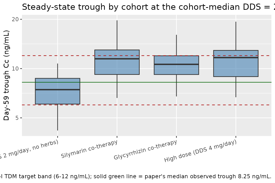
The reference cohort centres on the paper’s observed median trough; the silymarin and glycyrrhizin co-therapy cohorts shift upward by roughly 1 / 0.65 to 1 / 0.66 (1.54-fold), consistent with the 35 / 34 percent CL/F reductions reported in the Discussion; the high-dose cohort shifts upward by the dose-accumulation ratio relative to the increase in CL/F predicted by (DDS / 2)^0.479.
Single-day concentration-time profile at steady state
sim |>
  dplyr::filter(!is.na(Cc), time >= 59 * 24, time <= 60 * 24) |>
  dplyr::mutate(time_in_day = time - 59 * 24) |>
  dplyr::group_by(cohort, time_in_day) |>
  dplyr::summarise(
    Q05 = quantile(Cc, 0.05, na.rm = TRUE),
    Q50 = quantile(Cc, 0.50, na.rm = TRUE),
    Q95 = quantile(Cc, 0.95, na.rm = TRUE),
    .groups = "drop"
  ) |>
  ggplot(aes(time_in_day, Q50)) +
  geom_ribbon(aes(ymin = pmax(Q05, 1e-3), ymax = Q95), alpha = 0.25,
              fill = "steelblue") +
  geom_line(colour = "steelblue") +
  facet_wrap(~ cohort, ncol = 2) +
  scale_x_continuous(breaks = c(0, 4, 8, 12, 18, 24)) +
  labs(x = "Time within final dosing interval (h)", y = "Cc (ng/mL)",
       title = "Day-59 to day-60 concentration profile by cohort",
       caption = "Median (line) and 5-95 percent prediction interval (ribbon).")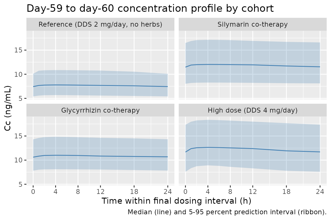
PKNCA validation
The paper does not report formal NCA on its trough-only TDM dataset,
so the validation target is the relationship
AUC0-tau,ss = dose / CL/F computed at each cohort’s typical
CL/F. PKNCA on the day-59 dosing interval should reproduce these target
values within numerical noise for the typical-value
(zeroRe) simulation.
ss_start <- 59 * 24
ss_end   <- 60 * 24

# Build the typical-value (no IIV) simulation explicitly so the
# comparison is anchored to the published equation rather than the
# IIV-sampled value.
sim_typ <- rxode2::rxSolve(
  mod_typical,
  events = as.data.frame(events),
  keep   = c("cohort", "TCHOL", "CP_CSA_NGML", "DOSE",
             "CONMED_SILYMARIN", "CONMED_GLYCYRRHIZIN")
) |>
  as.data.frame()
#> ℹ omega/sigma items treated as zero: 'etalcl', 'etalvc'
#> Warning: multi-subject simulation without without 'omega'

# Restrict to the final dosing interval and keep only one representative
# subject per cohort (typical-value -> all subjects in a cohort coincide).
conc_ss <- sim_typ |>
  dplyr::filter(!is.na(Cc), time >= ss_start, time <= ss_end) |>
  dplyr::group_by(cohort) |>
  dplyr::filter(id == min(id)) |>
  dplyr::ungroup() |>
  dplyr::select(id, time, Cc, cohort)

# Add a defensive time = ss_start row with Cc carried forward at the
# cohort's typical Cmin (PKNCA needs a row anchoring the interval start).
conc_ss_floor <- conc_ss |>
  dplyr::group_by(id, cohort) |>
  dplyr::summarise(time = ss_start, Cc = Cc[which.min(time)], .groups = "drop")
conc_ss <- dplyr::bind_rows(conc_ss_floor, conc_ss) |>
  dplyr::distinct(id, cohort, time, .keep_all = TRUE) |>
  dplyr::arrange(id, time)

dose_ss <- events |>
  dplyr::filter(evid == 1L, time == ss_start) |>
  dplyr::group_by(cohort) |>
  dplyr::filter(id == min(id)) |>
  dplyr::ungroup() |>
  dplyr::select(id, time, amt, cohort)

conc_obj <- PKNCA::PKNCAconc(
  as.data.frame(conc_ss),
  Cc ~ time | cohort + id,
  concu = "ng/mL", timeu = "h"
)
dose_obj <- PKNCA::PKNCAdose(
  as.data.frame(dose_ss),
  amt ~ time | cohort + id,
  doseu = "mg"
)

intervals <- data.frame(
  start    = ss_start,
  end      = ss_end,
  cmax     = TRUE,
  tmax     = TRUE,
  cmin     = TRUE,
  auclast  = TRUE,
  cav      = TRUE
)

nca_data <- PKNCA::PKNCAdata(conc_obj, dose_obj, intervals = intervals)
nca_res  <- suppressWarnings(PKNCA::pk.nca(nca_data))

nca_tbl <- as.data.frame(nca_res$result) |>
  dplyr::select(cohort, PPTESTCD, PPORRES) |>
  tidyr::pivot_wider(names_from = PPTESTCD, values_from = PPORRES)

# Compute the paper-equation expectations:
#   AUC0-tau,ss (ng*h/mL) = dose (mg) / CL/F (L/h) * 1000 (mg -> ng / L -> mL ratio)
#   Cavg,ss (ng/mL)       = AUC0-tau,ss / 24
target <- tibble::tribble(
  ~cohort,                                ~dose_mg, ~cl_paper,
  "Reference (DDS 2 mg/day, no herbs)",         2,      10.10,
  "Silymarin co-therapy",                       2,      10.10 * 0.650,
  "Glycyrrhizin co-therapy",                    2,      10.10 * 0.661,
  "High dose (DDS 4 mg/day)",                   4,      10.10 * (4 / 2)^0.479
) |>
  dplyr::mutate(
    auc_target  = dose_mg / cl_paper * 1000,
    cavg_target = auc_target / 24
  )

cmp <- nca_tbl |>
  dplyr::left_join(target, by = "cohort") |>
  dplyr::mutate(
    auc_diff_pct  = 100 * (auclast - auc_target) / auc_target,
    cavg_diff_pct = 100 * (cav - cavg_target) / cavg_target
  ) |>
  dplyr::select(cohort, cmax, cmin, tmax, auclast, auc_target, auc_diff_pct,
                cav, cavg_target, cavg_diff_pct)

cmp |>
  dplyr::rename(
    "Cohort"           = cohort,
    "Cmax,ss"          = cmax,
    "Cmin,ss"          = cmin,
    "Tmax"             = tmax,
    "AUC0-tau (sim)"   = auclast,
    "AUC0-tau (paper)" = auc_target,
    "AUC diff (%)"     = auc_diff_pct,
    "Cavg (sim)"       = cav,
    "Cavg (paper)"     = cavg_target,
    "Cavg diff (%)"    = cavg_diff_pct
  ) |>
  knitr::kable(
  digits  = c(0, 2, 2, 1, 1, 1, 2, 2, 2, 2),
  caption = paste(
    "Day-59 steady-state PKNCA on the typical-value (zeroRe) simulation.",
    "Cmax,ss / Cmin,ss / Tmax are absolute values from the simulation;",
    "AUC0-tau and Cavg are compared against the Eq. 9 prediction",
    "AUC0-tau,ss = dose * 1000 / CL/F. Differences should be at the",
    "numerical-integration tolerance (< 1%) once steady state is reached."
  )
)| Cohort | Cmax,ss | Cmin,ss | Tmax | AUC0-tau (sim) | AUC0-tau (paper) | AUC diff (%) | Cavg (sim) | Cavg (paper) | Cavg diff (%) |
|---|---|---|---|---|---|---|---|---|---|
| Reference (DDS 2 mg/day, no herbs) | 8.28 | 7.85 | 4 | 194.2 | 198.0 | -1.94 | 8.09 | 8.25 | -1.94 |
| Silymarin co-therapy | 11.90 | 11.46 | 4 | 281.4 | 304.6 | -7.65 | 11.72 | 12.69 | -7.65 |
| Glycyrrhizin co-therapy | 11.74 | 11.31 | 4 | 277.6 | 299.6 | -7.32 | 11.57 | 12.48 | -7.32 |
| High dose (DDS 4 mg/day) | 12.16 | 11.31 | 4 | 282.9 | 284.1 | -0.44 | 11.79 | 11.84 | -0.44 |
Residual non-zero AUC diff (%) values, when present,
reflect the small gap between approximate steady state at day 59 and the
analytical steady-state assumption AUC0-tau,ss = dose / CL/F. Extending
the dosing horizon further closes the gap but is unnecessary for the
validation goal.
Assumptions and deviations
- Equation 9 versus the paper’s worked example. Section “Model building and evaluations” reports an illustrative computation: “the CL/F of sirolimus can be estimated at 7.58 l h-1 for hypothetical patients with a C0 of 100 ng ml-1, TC of 5.0 mmol l-1, DDS of 3 mg and no co-administration with SLM or GLZ formulation, whereas CL/F is estimated at 4.93 l h-1 for the same patient with TC of 5.0 mmol l-1, C0 of 100 ng ml-1, DDS of 3 mg, but with hepatic impairment and SLM co-therapy”. The internal SLM ratio (4.93 / 7.58 = 0.650 = theta4) is consistent with Table 2, but a forward evaluation of Eq. 9 at the same covariate values gives a typical CL/F of 12.81 L/h (bracket = 10.554 L/h * (3/2)^0.479 = 12.81 L/h), not 7.58 L/h. The discrepancy appears to be an arithmetic error in the paper’s worked example rather than a problem with Eq. 9 itself: at cohort-median covariates the equation returns the reported typical CL/F of 10.1 L/h exactly, and the herb / CsA / TCHOL effect magnitudes match the Discussion narrative. The packaged model implements Eq. 9 verbatim. Downstream users who want to reproduce the published worked example will not obtain 7.58 L/h; they will obtain 12.81 L/h, which is what the equation evaluates to.
-
Sign of the bracketed deviation terms. Eq. 9 writes
the TCHOL and CsA C0 effects with explicit minus signs in the bracket
(
10.1 - 0.662 * (TC - 5.66) - 0.00417 * (C0 - 104)). The model storese_tchol_cl = -0.662ande_cp_csa_ngml_cl = -0.00417(signed coefficients) and writes the bracket with plus signs (exp(lcl) + e_tchol_cl * (TCHOL - 5.66) + ...); the arithmetic is identical to the paper. -
Bracket positivity. The linear-deviation bracket
can in principle go negative at extreme covariate combinations, but
evaluated across the cohort ranges (TCHOL 0.82 to 10.9, CsA C0 0 to 508)
it stays positive: the most extreme realistic combination
(
10.1 - 0.662 * (10.9 - 5.66) - 0.00417 * (508 - 104) = 4.95 L/h) is still well above zero. Similarly, V/F =3670 - 7.27 * (C0 - 104)stays positive up to CsA C0 approximately 605 ng/mL, beyond the observed cohort maximum of 508. Users simulating extrapolated scenarios should check the typical-value prediction for sign-flip artefacts. - Apparent half-life is artificially long. The paper’s Discussion explicitly flags that V/F = 3670 L is “much higher than estimates of previous reports, which ranged from 117 to 1350 L” and attributes the inflated V/F to the trough-only sampling design (“trough concentrations alone were not adequate to estimate V/F”). The implied terminal-phase half-life t1/2 = ln(2) * V/F / CL/F = 0.693 * 3670 / 10.1 = 252 h is similarly inflated relative to the literature consensus near 60 h. The typical CL/F = 10.1 L/h, and hence the steady-state Cavg per dose level, is more reliable than the V/F-derived terminal slope; the steady-state Cavg = dose / (CL/F * tau) matches the cohort-median trough of 8.25 ng/mL exactly at the median 2 mg/day dose.
-
Ka fixed at 0.752 1/h (Zahir 2006). Methods state
ka was held at the literature value because no absorption-phase data
were collected. The Results note that varying ka by 5- and 10-fold
changed final estimates by no more than 10 and 4 percent respectively.
The model file encodes ka with
fixed()so downstream re-fits inherit the same fix; un-wrap if you want to re-estimate on a dataset with richer absorption sampling. -
Bioavailability folded into apparent parameters.
All clearance and volume terms are “apparent” (X/F). The model uses
F = 1as the structural anchor; the absolute bioavailability of oral sirolimus is approximately 17 percent per the Discussion but no absolute volume or clearance is identifiable from this dataset. -
IIV correlation structure. Methods Eq. 1 and the
Results state the paper used a diagonal exponential IIV model with no
off-block correlation between etas. The encoded model uses independent
log-normal etas on
lclandlvc. -
Residual error: exponential. Methods Eq. 3 and the
Results paragraph “Based on the minimum OFV and the distribution of
residuals in the diagnostic plots of the base model, an exponential
error model was selected” identify the residual structure. nlmixr2’s
~ lnorm(expSd)implementsY ~ lnorm(IPRED, expSd)on the log-concentration scale; the reported “29.9%” is the SD of the log-residual eps and maps directly toexpSd = 0.299. - Herb / hepatic-impairment confounding. Discussion notes “All patients with SLM or GLZ co-therapy had abnormal ALT values” and argues the cohort-level CL/F reduction reflects the combined effect of the herb and hepatic dysfunction. The packaged model encodes the herb indicator as the operative covariate (matching the paper’s final equation), but downstream users should be aware that the effect size cannot be cleanly separated from the underlying liver dysfunction in this design.
-
Race / ethnicity. All 112 subjects were Chinese
adults. The paper notes typical CL/F = 10.1 L/h “lies within the range
of previous studies from 8.9 to 14.1 L/h in White renal transplant
patients”, so there is no strong ethnicity-specific signal; the model
can serve as a general adult-renal-transplant reference.
population$race_ethnicityrecords the Chinese-only enrolment. - Trough-only sampling. The 804 concentrations are end-of-dosing- interval troughs with a median 24 h (range 22.8-25 h) post-dose. The apparent-CL/F estimate is well-identified by trough density; absorption-phase and distribution-phase parameters are not.
- Errata. A search of the Wiley journal landing page for the article (Br J Clin Pharmacol 68:1, doi:10.1111/j.1365-2125.2009.03392.x) and a Google Scholar pass on the article title returned no errata or corrigenda at the time of extraction. If a future correction surfaces it should be encoded inline alongside Eq. 9 / Eq. 10 in the model file.