Danofloxacin in Yellow River carp (Song 2022) • nlmixr2lib

Model and source

#> ℹ parameter labels from comments will be replaced by 'label()'

Citation: Song Z-W, Yang F, Dai Y, Zhang C-S, Shao H-T, Wang H, Ma K-L, Li Z-E, Yang F. (2022). Population Pharmacokinetics of Danofloxacin in Yellow River Carp (Cyprinus carpio haematopterus) After One Single Oral Dose. Frontiers in Veterinary Science 9:868966. doi:10.3389/fvets.2022.868966.
Article: https://doi.org/10.3389/fvets.2022.868966
Open access full text (PMC): https://www.ncbi.nlm.nih.gov/pmc/articles/PMC9019490/

Veterinary (Yellow River carp, Cyprinus carpio haematopterus). One-compartment population PK model with first-order absorption and no absorption lag for danofloxacin after a single 10 mg/kg body-weight oral (gavage) dose in Yellow River carp held at 23.7 +/- 1.2 degC. Song 2022 fitted 24 sparsely sampled fish (four plasma samples each, drawn from a 16-point 0.25-144 h grid) in Phoenix NLME 8.1 with FOCE-ELS. The dose, V/F and CL/F are body-weight normalised in the source (dose in mg/kg, tvV in L/kg, tvCL in L/h/kg), so the model is driven with amt in mg/kg and returns Cc in ug/mL. Final model (Model 3, Table 5): tvKa 2.48 1/h, tvV 47.8 L/kg, tvCL 0.694 L/h/kg, exponential between-fish variability on all three (omega^2 = 3.45, 1.19 and 0.712) and a multiplicative residual error of 0.339. Model 3 keeps body weight as a power covariate on Ka, V/F and CL/F, centred on 0.38 kg (Eq. 1), but the three exponents are ‘results not shown’ in the paper; they are carried here as placeholders held at 0, so the model reproduces the published typical fish at every weight. The authors also fitted correlations between the three etas but did not print them, so the etas are independent here. See the vignette for both gaps.

Song 2022 is, in the authors’ words, the first population PK analysis of danofloxacin in Yellow River carp. Danofloxacin is a veterinary fluoroquinolone; the paper’s practical conclusion is that a single 10 mg/kg oral dose gives AUC/MIC and Cmax/MIC ratios above the fluoroquinolone targets (125 and 10) for pathogens with an MIC of at most 0.016 ug/mL.

Population

Thirty healthy Yellow River carp (Cyprinus carpio haematopterus) were bought from a commercial farm; 24 were dosed (four tanks of six) and six served as undosed controls supplying blank plasma (Animals section). Mean body weight was 0.38 kg (range 0.25 to 0.54 kg; per-fish weights are listed in Table 1). Fish were held at 23.7 +/- 1.2 degC after at least 7 days of acclimation.

Each fish received a single 10 mg/kg body-weight oral gavage of danofloxacin mesylate (5 mg/mL in saline) and was sampled sparsely, four times, from the tail vein, so that the 24 fish together cover 16 nominal times from 0.25 to 144 h. Plasma danofloxacin was measured by HPLC with fluorescence detection (LOQ 0.005 ug/mL).

str(ui$population)
#> List of 14
#>  $ species          : chr "Yellow River carp (Cyprinus carpio haematopterus)"
#>  $ n_subjects       : int 24
#>  $ n_studies        : int 1
#>  $ weight_range     : chr "0.25-0.54 kg"
#>  $ weight_mean      : chr "0.38 kg"
#>  $ dose_range       : chr "single 10 mg/kg body weight oral gavage (danofloxacin mesylate, 5 mg/mL in saline)"
#>  $ disease_state    : chr "healthy"
#>  $ regions          : chr "China (Henan University of Science and Technology, Luoyang)"
#>  $ water_temperature: chr "23.7 +/- 1.2 degC"
#>  $ water_quality    : chr "pH ~7.3; dissolved oxygen > 8 mg/L; ammonia ~0.1 mg/L"
#>  $ design           : chr "30 fish; 24 dosed fish in four equal tanks and 6 undosed controls supplying blank plasma. At least 7 days of ac"| __truncated__
#>  $ sampling         : chr "Sparse: each dosed fish sampled 4 times from the tail vein. Table 1 cycles four schedules across the 24 fish: ("| __truncated__
#>  $ bioanalysis      : chr "HPLC with fluorescence detection (ex 280 nm, em 450 nm); calibration 0.005-2 ug/mL, LOQ 0.005 ug/mL, mean recov"| __truncated__
#>  $ notes            : chr "Per-fish weights are in Table 1. Only one water temperature was studied, and the Discussion notes that fluoroqu"| __truncated__

Study design (Song 2022 Table 1)

# Song 2022 Table 1: per-fish body weight, in printed ID order. Four
# four-point schedules cycle across fish 1..24.
schedules <- list(
  A = c(0.25, 4, 16, 72),
  B = c(0.5, 6, 24, 96),
  C = c(1, 8, 36, 120),
  D = c(2, 12, 48, 144)
)
table1 <- tibble::tibble(
  id = 1:24,
  WT = c(
    0.40, 0.37, 0.35, 0.49, 0.31, 0.39, 0.25, 0.41, 0.37, 0.33, 0.37, 0.37,
    0.37, 0.32, 0.37, 0.41, 0.29, 0.53, 0.25, 0.40, 0.42, 0.54, 0.43, 0.37
  ),
  schedule = rep(names(schedules), times = 6)
)
nominal_times <- c(0.25, 0.5, 1, 2, 4, 6, 8, 12, 16, 24, 36, 48, 72, 96, 120, 144)
stopifnot(
  nrow(table1) == 24L,
  all(lengths(schedules) == 4L),
  setequal(unlist(schedules, use.names = FALSE), nominal_times),
  # Animals section: mean 0.38 kg, range 0.25-0.54 kg. 0.38 is also the
  # centring weight of Eq. 1.
  min(table1$WT) == 0.25, max(table1$WT) == 0.54,
  round(mean(table1$WT), 2) == 0.38
)
c(n_fish = nrow(table1), n_samples = nrow(table1) * 4L, mean_WT = round(mean(table1$WT), 4))
#>    n_fish n_samples   mean_WT 
#>   24.0000   96.0000    0.3796

Source trace

Every value below also carries an in-file comment next to its ini() entry in inst/modeldb/specificDrugs/Song_2022_danofloxacin_carp.R.

Equation / parameter	Value	Source location
`lka` (tvKa)	2.48 1/h	Table 5, Model 3; SE 0.123, CI 2.24 to 2.73
`lvc` (tvV, V/F)	47.8 L/kg	Table 5, Model 3; SE 1.90, CI 44.0 to 51.6
`lcl` (tvCL, CL/F)	0.694 L/h/kg	Table 5, Model 3; SE 0.012, CI 0.669 to 0.718
`e_wt_ka`, `e_wt_vc`, `e_wt_cl`	0 (placeholders)	Eq. 1 and the text after it: `dKadwt` is “results not shown”; V and CL “by the same algorithm”
`(WT / 0.38)^e` power form, 0.38 kg centre	n/a	Eq. 1 and the text after it (“the average body weight of all animals is 0.38 kg”)
`etalka` variance	3.45	Table 5, Model 3, “Interindividual variation omega^2 (CV%)” column
`etalvc` variance	1.19	Table 5, same column
`etalcl` variance	0.712	Table 5, same column
`propSd`	0.339	Table 5, Model 3 residual error; multiplicative error model per the Population Pharmacokinetic Modeling section
One compartment, first-order oral absorption, no lag	n/a	Population Pharmacokinetic Modeling (“single compartment extravascular administration”)
K10 = tvCL/tvV, T1/2 = ln2/K10, AUC0-inf = Dose/tvCL	n/a	Eqs. 2 to 4; results in Table 2
Dose 10 mg/kg BW, single oral gavage	n/a	Drug Administration and Sampling

Models 1 (no covariates) and 2 (body weight) in Table 5 are intermediate steps; the packaged model is the final Model 3 that the authors used for every reported result.

What the bracketed numbers in Table 5 are

The abstract calls the bracketed omega values (0.203%, 8.40%, 4.35%) the “coefficient of variation between individuals”. They are relative standard errors. In this paper the “CV%” of an estimate is its SE divided by the estimate, as the fixed-effect rows show, and a log-normal variance of 3.45 would mean a between-fish CV of several hundred percent, not 0.2%:

# Song 2022 Table 5, Model 3: (estimate, SE, printed CV%) for the fixed effects
fx <- tibble::tribble(
  ~parameter, ~estimate, ~se, ~cv_printed,
  "tvKa", 2.48, 0.123, 4.94,
  "tvV", 47.8, 1.90, 3.97,
  "tvCL", 0.694, 0.012, 1.77,
  "Residual error", 0.339, 0.014, 4.06
) |>
  mutate(se_over_estimate = 100 * se / estimate)
# The SEs are printed to 2-3 significant figures, so 100*SE/estimate
# matches the printed CV% to within that rounding.
stopifnot(all(abs(fx$se_over_estimate - fx$cv_printed) < 0.2))
# Log-normal CV implied by each omega^2, if the leading number were a CV it
# would not be this.
cv_lognormal <- 100 * sqrt(exp(c(3.45, 1.19, 0.712)) - 1)
stopifnot(all(cv_lognormal > 90))
fx
#> # A tibble: 4 × 5
#>   parameter      estimate    se cv_printed se_over_estimate
#>   <chr>             <dbl> <dbl>      <dbl>            <dbl>
#> 1 tvKa              2.48  0.123       4.94             4.96
#> 2 tvV              47.8   1.9         3.97             3.97
#> 3 tvCL              0.694 0.012       1.77             1.73
#> 4 Residual error    0.339 0.014       4.06             4.13
round(cv_lognormal)
#> [1] 552 151 102

So the leading number in the omega column is the variance used in the model, and the bracketed number is its RSE.

Reproducing the secondary parameters (Table 2)

Table 2 gives K10 = 0.015 1/h, T1/2 = 47.7 h and AUC0-inf = 14.4 h*ug/mL, computed from the typical values by Eqs. 2 to 4. Solving the packaged ODE model at its typical values for a 0.38 kg fish and running PKNCA on the result checks the ODE structure, the dosing route, the body-weight-normalised units and the transcribed values against those three numbers.

mod <- readModelDb("Song_2022_danofloxacin_carp")
mod_typical <- rxode2::zeroRe(mod)
#> ℹ parameter labels from comments will be replaced by 'label()'

# Fine early grid for the peak, then out to 720 h (about 15 half-lives) so the
# AUC extrapolation is a small correction.
grid_typical <- sort(unique(c(seq(0, 24, by = 0.05), seq(24, 720, by = 2))))
ev_typical <- rxode2::et(amt = 10, cmt = "depot") |>
  rxode2::et(grid_typical) |>
  as.data.frame() |>
  mutate(WT = 0.38)

sim_typical <-
  rxode2::rxSolve(mod_typical, ev_typical, returnType = "data.frame") |>
  mutate(id = 1L, treatment = "10 mg/kg")
#> ℹ omega/sigma items treated as zero: 'etalka', 'etalvc', 'etalcl'
stopifnot(all(sim_typical$Cc >= 0))

#> Warning in scale_y_log10(): log-10 transformation introduced infinite values.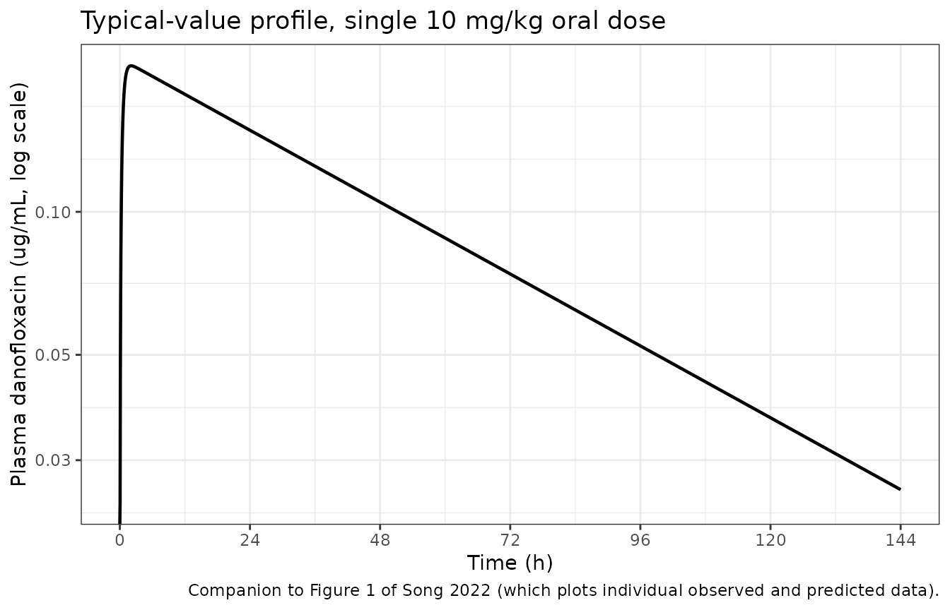

PKNCA validation

nca_conc <- sim_typical |>
  dplyr::filter(!is.na(Cc)) |>
  dplyr::select(id, time, Cc, treatment)
nca_conc <- dplyr::bind_rows(
  nca_conc,
  nca_conc |> dplyr::distinct(id, treatment) |> dplyr::mutate(time = 0, Cc = 0)
) |>
  dplyr::distinct(id, treatment, time, .keep_all = TRUE) |>
  dplyr::arrange(id, treatment, time)

conc_obj <- PKNCA::PKNCAconc(nca_conc, Cc ~ time | treatment + id)
dose_df <- data.frame(id = 1L, time = 0, amt = 10, treatment = "10 mg/kg")
dose_obj <- PKNCA::PKNCAdose(dose_df, amt ~ time | treatment + id)
intervals <- data.frame(
  start = 0, end = Inf,
  cmax = TRUE, tmax = TRUE, auclast = TRUE,
  aucinf.obs = TRUE, half.life = TRUE, lambda.z = TRUE
)
nca_res <- PKNCA::pk.nca(PKNCA::PKNCAdata(conc_obj, dose_obj, intervals = intervals))

nca_wide <- as.data.frame(nca_res) |>
  dplyr::select(PPTESTCD, PPORRES) |>
  tidyr::pivot_wider(names_from = PPTESTCD, values_from = PPORRES)
nca_wide[, c("cmax", "tmax", "auclast", "aucinf.obs", "half.life", "lambda.z")]
#> # A tibble: 1 × 6
#>    cmax  tmax auclast aucinf.obs half.life lambda.z
#>   <dbl> <dbl>   <dbl>      <dbl>     <dbl>    <dbl>
#> 1 0.203   2.1    14.4       14.4      47.7   0.0145

Gate 1 – Table 2 secondary parameters

auc_sim <- nca_wide$aucinf.obs
thalf_sim <- nca_wide$half.life
k10_sim <- nca_wide$lambda.z
pct <- function(sim, ref) (sim - ref) / ref * 100

# Deterministic typical-value solve, so the tolerance only has to absorb
# the 3-significant-figure printing of Table 2 and PKNCA's numerical AUC.
# A 10% error in a transcribed clearance, volume, dose or unit moves these
# by 10% or more.
stopifnot(
  abs(pct(auc_sim, 14.4)) < 1,
  abs(pct(thalf_sim, 47.7)) < 1,
  round(k10_sim, 3) == 0.015
)

tibble::tibble(
  Quantity = c("AUC0-inf (h*ug/mL)", "T1/2 (h)", "K10 (1/h)"),
  `Song 2022 Table 2` = c(14.4, 47.7, 0.015),
  Simulated = signif(c(auc_sim, thalf_sim, k10_sim), 4),
  `% diff` = round(pct(c(auc_sim, thalf_sim, k10_sim), c(14.4, 47.7, 0.015)), 2)
) |>
  knitr::kable(caption = "Gate 1: PKNCA on the typical-value solve vs Song 2022 Table 2.")

Gate 1: PKNCA on the typical-value solve vs Song 2022 Table 2.
Quantity	Song 2022 Table 2	Simulated	% diff
AUC0-inf (h*ug/mL)	14.400	14.41000	0.06
T1/2 (h)	47.700	47.74000	0.09
K10 (1/h)	0.015	0.01452	-3.21

Comparison against the published NCA

# Table 2 holds the model-derived AUC0-inf and T1/2, the like-for-like
# reference for a typical-value simulation. The only published Cmax and Tmax
# are from Table 4, a naive-pooled NCA of the sparse data that the authors
# used only to seed initial estimates; they are shown for context and are
# expected to differ.
published <- tibble::tribble(
  ~treatment, ~cmax, ~tmax, ~aucinf.obs, ~half.life,
  "10 mg/kg", 0.166, 10.6, 14.4, 47.7
)
simulated <- nca_wide |>
  dplyr::mutate(treatment = "10 mg/kg") |>
  dplyr::select(treatment, cmax, tmax, aucinf.obs, half.life)

cmp <- nlmixr2lib::ncaComparisonTable(
  simulated = simulated,
  reference = published,
  by = "treatment",
  units = c(cmax = "ug/mL", tmax = "h", aucinf.obs = "h*ug/mL", half.life = "h"),
  tolerance_pct = 20
)
knitr::kable(
  cmp,
  caption = paste(
    "Simulated (typical value) vs published values.",
    "AUC0-inf and T1/2 are from Table 2 (model-derived);",
    "Cmax and Tmax are from Table 4 (naive-pooled NCA).",
    "* differs from reference by >20%."
  )
)

Simulated (typical value) vs published values. AUC0-inf and T1/2 are from Table 2 (model-derived); Cmax and Tmax are from Table 4 (naive-pooled NCA). * differs from reference by >20%.
NCA parameter	treatment	Reference	Simulated	% diff
Cmax (ug/mL)	10 mg/kg	0.166	0.203	+22.3%*
Tmax (h)	10 mg/kg	10.6	2.1	-80.2%*
AUC0-∞ (obs) (h*ug/mL)	10 mg/kg	14.4	14.4	+0.1%
t½ (h)	10 mg/kg	47.7	47.7	+0.1%

attr(cmp, "footnote")
#> [1] "* differs from reference by more than ±20%."

The Cmax and Tmax rows are flagged, as expected. The typical-value curve peaks at about 0.20 ug/mL near 2 h, while the naive-pooled NCA of Table 4 reports a mean Cmax of 0.166 ug/mL at 10.6 h with SDs (0.321 and 14.5 h) larger than the means themselves. Table 4’s AUC0-inf (4.48) is also a third of the model-derived 14.4. The Discussion calls these NCA values “a lousy prediction ability” and uses them only as initial estimates, so they are not a validation target.

Gate 2 – the PK/PD ratios in the Discussion

The Discussion reports AUC/MIC = 900 and Cmax/MIC = 10.4 at an MIC of 0.016 ug/mL. AUC/MIC is 14.4 / 0.016 = 900, the model-derived AUC; Cmax/MIC is 0.166 / 0.016 = 10.4, the naive-pooled Table 4 Cmax. Recomputing the AUC ratio from the packaged model checks it against the published conclusion.

mic <- 0.016
auc_mic_model <- auc_sim / mic
stopifnot(
  abs(pct(auc_mic_model, 900)) < 1,
  # The published Cmax/MIC uses Table 4's naive-pooled Cmax, not a model value.
  round(0.166 / mic, 1) == 10.4,
  # The conclusion (both targets met at MIC 0.016) holds with the model Cmax too.
  auc_mic_model >= 125, nca_wide$cmax / mic >= 10
)
c(
  `AUC/MIC (model)` = round(auc_mic_model),
  `Cmax/MIC (model typical value)` = round(nca_wide$cmax / mic, 1),
  `Cmax/MIC (paper, Table 4 Cmax)` = round(0.166 / mic, 1)
)
#>                AUC/MIC (model) Cmax/MIC (model typical value) 
#>                          901.0                           12.7 
#> Cmax/MIC (paper, Table 4 Cmax) 
#>                           10.4

Between-fish variability

Song 2022 publishes no VPC; Figure 1 overlays individual observed and predicted concentrations, and the observed data are not tabulated. The cohort below draws 200 fish with body weights resampled from Table 1 and shows the predicted 5th, 50th and 95th percentiles over the 144 h sampling window.

# rxSetSeed() fixes rxode2's stream per solver thread but not across thread
# counts, so the assertions below hold for any cohort this model can draw.
rxode2::rxSetSeed(20220406)
set.seed(20220406) # for the base-R weight resampling
n_fish <- 200L
grid_cohort <- sort(unique(c(seq(0, 24, by = 0.25), seq(26, 144, by = 2))))
wt_draw <- tibble::tibble(id = seq_len(n_fish), WT = sample(table1$WT, n_fish, replace = TRUE))
ev_cohort <- rxode2::et(amt = 10, cmt = "depot") |>
  rxode2::et(grid_cohort) |>
  rxode2::et(id = seq_len(n_fish)) |>
  as.data.frame() |>
  left_join(wt_draw, by = "id")

sim_cohort <- rxode2::rxSolve(mod, ev_cohort, returnType = "data.frame")
#> ℹ parameter labels from comments will be replaced by 'label()'
stopifnot(dplyr::n_distinct(sim_cohort$id) == n_fish)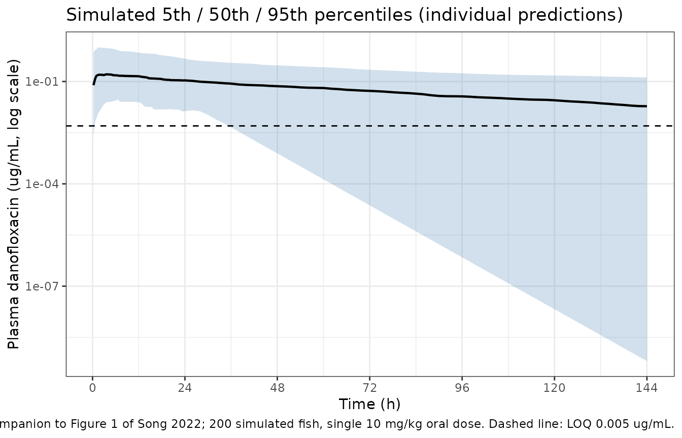

Gate 3 – the omega diagonal reproduces as encoded

per_fish <- sim_cohort |>
  group_by(id) |>
  summarise(ka = first(ka), vc = first(vc), cl = first(cl), .groups = "drop")

realised <- tibble::tibble(
  parameter = c("ka", "vc", "cl"),
  encoded_median = c(2.48, 47.8, 0.694),
  encoded_omega = sqrt(c(3.45, 1.19, 0.712)),
  cohort_median = c(median(per_fish$ka), median(per_fish$vc), median(per_fish$cl)),
  cohort_sd_log = c(sd(log(per_fish$ka)), sd(log(per_fish$vc)), sd(log(per_fish$cl)))
) |>
  mutate(
    median_log_ratio = log(cohort_median / encoded_median),
    sd_diff = cohort_sd_log - encoded_omega
  )

# Cohort statistics: SE(log median) ~= 1.2533 * omega / sqrt(n) = 0.165 at
# worst (ka, omega 1.86), SE(SD) ~= omega / sqrt(2n) = 0.093. The bounds sit
# at about 5 SE and still go red on a variance-vs-SD or decimal-point error,
# which shifts these by 0.5 or more on ka.
stopifnot(
  max(abs(realised$median_log_ratio)) < 0.85,
  max(abs(realised$sd_diff)) < 0.45
)

realised |>
  mutate(across(where(is.numeric), \(x) round(x, 3))) |>
  dplyr::rename(
    "Parameter" = parameter,
    "Encoded median" = encoded_median,
    "Encoded omega" = encoded_omega,
    "Cohort median" = cohort_median,
    "Cohort SD(log)" = cohort_sd_log,
    "log(median ratio)" = median_log_ratio,
    "SD difference" = sd_diff
  ) |>
  knitr::kable(caption = "Gate 3: realised cohort vs the encoded log-normal IIV.")

Gate 3: realised cohort vs the encoded log-normal IIV.
Parameter	Encoded median	Encoded omega	Cohort median	Cohort SD(log)	log(median ratio)	SD difference
ka	2.480	1.857	2.295	1.982	-0.077	0.125
vc	47.800	1.091	47.879	1.110	0.002	0.019
cl	0.694	0.844	0.641	0.956	-0.079	0.112

The body-weight placeholders

With the three exponents held at 0, body weight has no effect: the typical fish at 0.25 kg and at 0.54 kg (the ends of the observed range) have the same profile. A user who obtains the authors’ estimates can set them with ini(); for example mod |> rxode2::ini(e_wt_cl = 0.75) would apply an exponent of 0.75 on CL/F (an arbitrary illustration, not a value from the paper).

ev_wt <- rxode2::et(amt = 10, cmt = "depot") |>
  rxode2::et(c(1, 2, 24, 72)) |>
  rxode2::et(id = 1:2) |>
  as.data.frame() |>
  mutate(WT = ifelse(id == 1, 0.25, 0.54))
sim_wt <- rxode2::rxSolve(mod_typical, ev_wt, returnType = "data.frame")
#> ℹ omega/sigma items treated as zero: 'etalka', 'etalvc', 'etalcl'
#> Warning: multi-subject simulation without without 'omega'
cc_wt <- tidyr::pivot_wider(sim_wt[, c("id", "time", "Cc")], names_from = id, values_from = Cc)
# Same parameters drawn from the same equations, so this is exact.
stopifnot(isTRUE(all.equal(cc_wt[["1"]], cc_wt[["2"]])))
cc_wt
#> # A tibble: 4 × 3
#>    time    `1`    `2`
#>   <dbl>  <dbl>  <dbl>
#> 1     1 0.190  0.190 
#> 2     2 0.203  0.203 
#> 3    24 0.149  0.149 
#> 4    72 0.0740 0.0740

Assumptions and deviations

The body-weight exponents are not published. Eq. 1 retains body weight as a power covariate on Ka, V/F and CL/F, centred on 0.38 kg, in the final model; the text calls the exponent “results not shown”, and no value appears anywhere in the paper (there is no supplement). The maintainers kept the published covariate structure with the three exponents (e_wt_ka, e_wt_vc, e_wt_cl) held at 0 as labelled placeholders. The typical values at 0.38 kg are complete and reproduce Table 2 exactly, so predictions for a fish of mean weight are as published. For other weights the model returns the mean-weight parameters; the observed range is narrow (0.25 to 0.54 kg), so the missing exponents move predictions only within about a factor of two in weight. The dose and V/F, CL/F are in any case expressed per kg body weight.
The omega off-diagonals are not published. Model 3 adds a “covariance model” over the three etas (the Discussion reports a Pearson correlation between them and an LRT of 35.9 against Model 2), but no covariance or correlation is printed. The etas are independent here. Typical-value results (Gates 1 and 2) are unaffected; cohort percentiles will differ from the authors’ by an amount that depends on the unknown correlations.
The bracketed omega numbers are RSEs, not between-fish CVs. Shown above from the paper’s own fixed-effect rows; the abstract’s wording is not followed.
Multiplicative residual error = proportional. Phoenix NLME’s multiplicative error model is C * (1 + eps), so the reported 0.339 is a proportional SD (propSd). Table 5’s “ug/ml” in the Units column for the residual error is not used.
Table 1 rows 21 to 24 are partly misaligned in the typeset table. Their weights (0.42, 0.54, 0.43, 0.37) are read in printed order; they reproduce the stated mean and range. The sampling schedule is assumed to continue the four-fish cycle of rows 1 to 20.
Observed data are not reproduced. No concentration table is published, so Figures 1 and 2 cannot be overlaid with observations.
Single temperature. All parameters apply at 23.7 +/- 1.2 degC; the Discussion notes that fluoroquinolone elimination in fish depends on water temperature.
No non-paper-derived parameter values. Every estimated ini() entry is transcribed from Song 2022 Table 5; nothing was digitised from a figure, obtained by correspondence or carried from an upstream model.