Secukinumab + ixekizumab skin IL-17A target engagement (Ayyar 2022)
Source:vignettes/articles/Ayyar_2022_il17a_target_engagement.Rmd
Ayyar_2022_il17a_target_engagement.RmdModel and source
Ayyar et al. (2022) combined a minimal physiologically based PK (mPBPK) model with model-based meta-analyses (MBMA) for the two marketed anti-IL-17A antibodies, secukinumab and ixekizumab. The aim was to predict free IL-17A suppression (target engagement, TE) in psoriatic skin and relate it to clinical response. The paper contributes four model files to the library:
| Model | Content |
|---|---|
Ayyar_2022_secukinumab_mpbpk |
mPBPK + quasi-equilibrium TMDD in serum and skin for secukinumab, plus the TE-based PASI75 / PASI90 MBMA |
Ayyar_2022_ixekizumab_mpbpk |
the same structure with the ixekizumab drug parameters |
Ayyar_2022_secukinumab_mbma |
dose-based PASI75 / PASI90 MBMA for secukinumab (Figure 2) |
Ayyar_2022_ixekizumab_mbma |
dose-based PASI75 / PASI90 MBMA for ixekizumab (Figure 2) |
- Citation: Ayyar VS, Lee JB, Wang W, Pryor M, Zhuang Y, Wilde T, Vermeulen A. Minimal Physiologically-Based Pharmacokinetic (mPBPK) Metamodeling of Target Engagement in Skin Informs Anti-IL17A Drug Development in Psoriasis. Front Pharmacol. 2022;13:862291. doi:10.3389/fphar.2022.862291
- Article: https://doi.org/10.3389/fphar.2022.862291 (open access)
- Supplementary Material: DataSheet1 (model equations) and DataSheet2 (NONMEM control stream for secukinumab), linked from the article page.
mod_sec <- rxode2::rxode2(readModelDb("Ayyar_2022_secukinumab_mpbpk"))
mod_ixe <- rxode2::rxode2(readModelDb("Ayyar_2022_ixekizumab_mpbpk"))
mbma_sec <- rxode2::rxode2(readModelDb("Ayyar_2022_secukinumab_mbma"))
mbma_ixe <- rxode2::rxode2(readModelDb("Ayyar_2022_ixekizumab_mbma"))
Population
All data came from published reports and regulatory reviews,
extracted as group means (Table 1 of the paper). Secukinumab data came
from the Phase 2 proof-of-concept study (FDA 2015, N = 36), the low
dose-ranging study (Papp 2013, N = 125), the high dose-ranging and
regimen-finding studies (Rich 2013, N = 100 and 404), the Phase 3
ERASURE, FIXTURE and FEATURE studies (N = 734, 974, 176), and the
open-flow microperfusion skin biodistribution study (Dragatin 2016).
Ixekizumab data came from the Phase 1 dose-escalation study (FDA 2016, N
= 46), the Phase 2 dose-ranging study (Leonardi 2012, N = 141) and the
Phase 3 UNCOVER-1/2/3 studies (Papp 2018). All participants were adults
with moderate-to-severe plaque psoriasis. Individual demographics were
not available. The mPBPK model was fitted in NONMEM 7.4 (FOCE-I) to mean
data (naive pooling) with the omega matrix fixed to zero, so the models
have no between-subject variability. The MBMAs were fitted by
nls to placebo-adjusted week-12 response rates. The same
information is in each model’s population metadata.
Model structure and units
The model follows Supplementary Eq. 1-12 and the $DES
block of the secukinumab control stream:
- An SC depot drains into plasma at
ka, with bioavailabilityF. - Free drug leaves plasma by convection into three interstitial
spaces: skin (
is_skin), muscle (is_muscle) and lumped leaky tissues (leaky). The flows areL * (1 - sigma). Drug returns throughlymphatL * (1 - sigma_L). - Free drug is cleared from plasma at the linear clearance
CL. - IL-17A binds drug under quasi-equilibrium (QE) in plasma and in skin
ISF, with the drug’s
KD. Total IL-17A followsdRtot/dt = ksyn - kdeg * (Rtot - AR) - kint * AR, whereARis the complex. The complex is eliminated atkint, so the total-drug states losekint * AR * V.
The paper reports KD and the IL-17A baselines in pM, and its QE
equations mix them with drug concentrations. The NONMEM model must
therefore have run in molar units. The models here take doses in
pmol and report every concentration in pM. The paper does not
state the antibody molecular weight. This vignette uses a nominal 150
kDa IgG (1 mg = 6667 pmol), the same convention as
Zheng_2020_CNTO5048_mouse_mpbpk, which comes from the same
group. Drug concentrations are converted back to ug/mL with the same
factor. With this factor the model reproduces the paper’s printed TE
values to the printed precision (below).
mw_mab <- 150000 # g/mol, nominal IgG (not stated in the paper)
mg_to_pmol <- function(mg) mg * 1e9 / mw_mab
pM_to_ugmL <- function(pM) pM * mw_mab / 1e9
# Empirical display factors for IL-17A, read from the paper's own figures.
# TOTAL IL-17A: the serum line of Figure 3E runs from about 2.8 pg/mL (baseline
# 0.015 pM) to about 100 pg/mL (plateau 0.54 pM), and the skin line of Figure
# 5B from about 50 to about 360 pg/mL (0.28 to 2.0 pM): about 185 pg/mL per pM.
# FREE IL-17A: the skin line of Figure 5A starts at about 10 pg/mL (0.28 pM)
# and the secukinumab 300 mg line sits at about 0.04 pg/mL at week 8 (0.0012
# pM): about 35 pg/mL per pM.
il17_total_pgmL_per_pM <- 185
il17_free_pgmL_per_pM <- 35
The two factors are used only to put IL-17A on the same pg/mL axes as the paper’s figures. They are not part of any model. 35 pg/mL per pM is the mass of the ~35 kDa IL-17A homodimer. 185 pg/mL per pM equals the mass of a 150 kDa antibody bound to IL-17A, as if total IL-17A (almost all of it complexed) had been converted with the complex mass.
Source trace
| Equation / parameter | Secukinumab | Ixekizumab | Source location |
|---|---|---|---|
| ODE system | – | – | Supplementary DataSheet1 Eq. 1-8; DataSheet2 $DES
|
| QE free drug, complex | – | – | DataSheet1 Eq. 9-12; DataSheet2 $DES
|
lcl (CL) |
0.154 L/day | 0.379 L/day | Table 2 (estimated) |
lfdepot (F) |
0.729 | 0.81 | Table 2 (fixed; popPK) |
lka (ka) |
0.18 1/day | 0.24 1/day | Table 2 (fixed; popPK) |
llymphflow (L) |
2.9 L/day | shared | Table 2 |
llymphflow_skin / _muscle /
_leaky
|
0.247 / 0.71 / 1.943 L/day | shared | Table 2 |
lvc (Vp) |
2.6 L | shared | Table 2 |
lvleaky (V2) |
4.368 L | shared | DataSheet2 THETA(9); Table 2 prints 4.37 |
lvskin / lvmuscle /
lvlymph
|
1.81 / 6.3 / 2.6 L | shared | Table 2 |
sigma_skin |
0.630 | 0.63 (fixed to secukinumab) | Table 2, footnote b |
sigma_muscle / sigma_l
|
0.95 / 0.2 | shared | Table 2 |
sigma_leaky |
0.363 | 0.524 | Table 2 (estimated for each drug) |
lkdeg / lkdeg_skin
|
45.5 / 2.44 1/day | shared | Table 2 |
lkint |
1.24 1/day | 1.24 (fixed to secukinumab) | Table 2, footnote b |
lkint_skin |
0.34 1/day | shared | Table 2 (= 2.5 x Ls / Vs) |
lr0 / lr0_skin
|
0.015 / 0.28 pM | shared | Table 2 |
ksyn (derived) |
0.683 pM/day | shared | Table 2; DataSheet2 $PK
|
lkd (KD) |
129 pM | 1.8 pM | Table 2 |
TE-MBMA PASI75 e0, emax,
ec50, hill
|
78.11, -26.94, 8.851 %, 1.094 | shared | Eq. 1; digitised Figure 6 |
TE-MBMA PASI90 e0, emax,
ec50, hill
|
66.46, -6.839, 3.062 %, 1.262 | shared | Eq. 1; digitised Figure 6 |
Dose-MBMA PASI75 e0, emax,
ed50, hill
|
-1.245, 75.82, 16.94 mg/wk, 1.898 | -7.944, 82.12, 2.605 mg/wk, 1.653 | Eq. 1; digitised Figure 2 |
Dose-MBMA PASI90 e0, emax,
ed50, hill
|
-0.821, 66.61, 36.91 mg/wk, 1.868 | -6.973, 68.56, 2.888 mg/wk, 1.474 | Eq. 1; digitised Figure 2 |
| Residual errors | not reported | not reported | Methods (proportional, on log concentrations) |
The paper prints none of the MBMA parameter values. The maintainers
digitised each trend line from the figure images in the article PDF and
refitted Eq. 1,
Response = E0 + x^hill * (Emax - E0) / (x^hill + E50^hill),
by nls to the digitised points. The refits reproduce the
digitised lines to within 1 percentage point (residual SD 0.14-0.9
points). The MBMA outputs are fractions on a 0-1 scale (the paper uses
percent).
Helpers
# One-subject event table: SC doses into the depot (pmol) and an observation
# grid. Observation rows carry no compartment; with several declared
# endpoints rxode2 then returns every output on each row.
make_events <- function(dose_mg, dose_day, obs_days, cmt = "depot", id = 1L) {
  doses <- data.frame(
    id = id, time = dose_day, amt = mg_to_pmol(dose_mg), cmt = cmt,
    evid = 1L, dvid = NA_integer_
  )
  obs <- data.frame(
    id = id, time = obs_days, amt = 0, cmt = NA_character_,
    evid = 0L, dvid = 1L
  )
  out <- rbind(doses, obs)
  out[order(out$time, -out$evid), ]
}

solve_regimen <- function(mod, dose_mg, dose_day, obs_days, label) {
  ev <- make_events(dose_mg, dose_day, obs_days)
  rxode2::rxSolve(mod, ev, returnType = "data.frame") |>
    dplyr::mutate(regimen = label)
}

# Approved-regimen dosing up to (not including) the week-12 read-out
sec_days <- c(0, 7, 14, 21, 28, 56) # weeks 0, 1, 2, 3, 4, then q4w
ixe_days <- c(0, 14, 28, 42, 56, 70) # 160 mg at week 0, then 80 mg q2w
grid12 <- seq(0, 84, by = 0.25)
Baseline steady state
Without drug, total IL-17A must stay at its baseline in both serum
and skin: ksyn = kdeg * R0 in each space.
nodose <- data.frame(
  id = 1L, time = c(0, 28, 84), amt = 0, cmt = NA_character_,
  evid = 0L, dvid = 1L
)
bl <- rxode2::rxSolve(mod_sec, nodose, returnType = "data.frame")
bl[, c("time", "Ctotal_target", "Ctotal_target_skin", "Cfree_target_skin")]
#>   time Ctotal_target Ctotal_target_skin Cfree_target_skin
#> 1    0         0.015               0.28              0.28
#> 2   28         0.015               0.28              0.28
#> 3   84         0.015               0.28              0.28
stopifnot(
  all(abs(bl$Ctotal_target / 0.015 - 1) < 1e-6),
  all(abs(bl$Ctotal_target_skin / 0.28 - 1) < 1e-6)
)
Target engagement at the approved regimens (Results, Figure 6)
The paper’s headline numbers are the 12-week average skin TE:
98.6% for secukinumab 300 mg at weeks 0, 1, 2, 3, 4
then q4w, and 99.9% for ixekizumab 160 mg then 80 mg
q2w (Results and Discussion). In other words, free skin IL-17A averaged
1.4% and 0.1% of baseline. Figure 6 also marks secukinumab 150 mg at
about 2.4% of baseline. Each model carries the running average as
free_target_skin_avg_pct, defined as the cumulative free
skin IL-17A divided by elapsed time. Its value at day 84 is the paper’s
metric.
sims12 <- dplyr::bind_rows(
  solve_regimen(mod_sec, rep(300, 6), sec_days, grid12, "Secukinumab 300 mg"),
  solve_regimen(mod_sec, rep(150, 6), sec_days, grid12, "Secukinumab 150 mg"),
  solve_regimen(mod_ixe, c(160, rep(80, 5)), ixe_days, grid12, "Ixekizumab 160/80 mg q2w")
)
te <- sims12 |>
  dplyr::filter(time == 84) |>
  dplyr::transmute(
    regimen,
    `Average free skin IL-17A (% baseline)` = round(free_target_skin_avg_pct, 3),
    `Average TE (%)` = round(te_skin_avg_pct, 2),
    `Published` = c("98.6% TE", "about 2.4% free (Figure 6 arrow)", "99.9% TE"),
    `PASI75 (placebo-adjusted)` = round(prob_pasi75_pbo_adj, 3),
    `PASI90 (placebo-adjusted)` = round(prob_pasi90_pbo_adj, 3)
  )
knitr::kable(te)| regimen | Average free skin IL-17A (% baseline) | Average TE (%) | Published | PASI75 (placebo-adjusted) | PASI90 (placebo-adjusted) |
|---|---|---|---|---|---|
| Secukinumab 300 mg | 1.381 | 98.62 | 98.6% TE | 0.659 | 0.468 |
| Secukinumab 150 mg | 2.376 | 97.62 | about 2.4% free (Figure 6 arrow) | 0.580 | 0.356 |
| Ixekizumab 160/80 mg q2w | 0.105 | 99.89 | 99.9% TE | 0.773 | 0.654 |
# The solve is deterministic (no random effects), so these bounds can be tight;
# they still leave room for the nominal 150 kDa molecular weight.
stopifnot(
  abs(te$`Average TE (%)`[1] - 98.6) < 0.1,
  abs(te$`Average free skin IL-17A (% baseline)`[2] - 2.4) < 0.25,
  abs(te$`Average TE (%)`[3] - 99.9) < 0.05
)
All three reproduce the paper. The TE result depends only weakly on the assumed molecular weight:
mw_sens <- lapply(c(140000, 150000, 160000), function(mw) {
  ev <- make_events(rep(300, 6), sec_days, 84)
  ev$amt[ev$evid == 1] <- 300 * 1e9 / mw
  s <- rxode2::rxSolve(mod_sec, ev, returnType = "data.frame")
  data.frame(`MW (kDa)` = mw / 1000, `Secukinumab 300 mg average TE (%)` = round(s$te_skin_avg_pct, 3), check.names = FALSE)
})
knitr::kable(do.call(rbind, mw_sens))| MW (kDa) | Secukinumab 300 mg average TE (%) |
|---|---|
| 140 | 98.691 |
| 150 | 98.619 |
| 160 | 98.547 |
Figure 5: skin IL-17A for the approved regimens
sims12 |>
  dplyr::select(time, regimen, Cfree_target_skin, Ctotal_target_skin) |>
  tidyr::pivot_longer(c(Cfree_target_skin, Ctotal_target_skin), names_to = "species", values_to = "pM") |>
  dplyr::mutate(
    species = dplyr::recode(species, Cfree_target_skin = "A: skin free IL-17A", Ctotal_target_skin = "B: skin total IL-17A"),
    pgmL = pM * ifelse(grepl("free", species), il17_free_pgmL_per_pM, il17_total_pgmL_per_pM)
  ) |>
  ggplot(aes(time / 7, pgmL, colour = regimen)) +
  geom_line(linewidth = 0.8) +
  facet_wrap(~species, scales = "free_y") +
  scale_y_log10() +
  labs(
    x = "Time (weeks)", y = "IL-17A (pg/mL)", colour = NULL,
    caption = "Replicates Figure 5 of Ayyar 2022."
  ) +
  theme(legend.position = "bottom")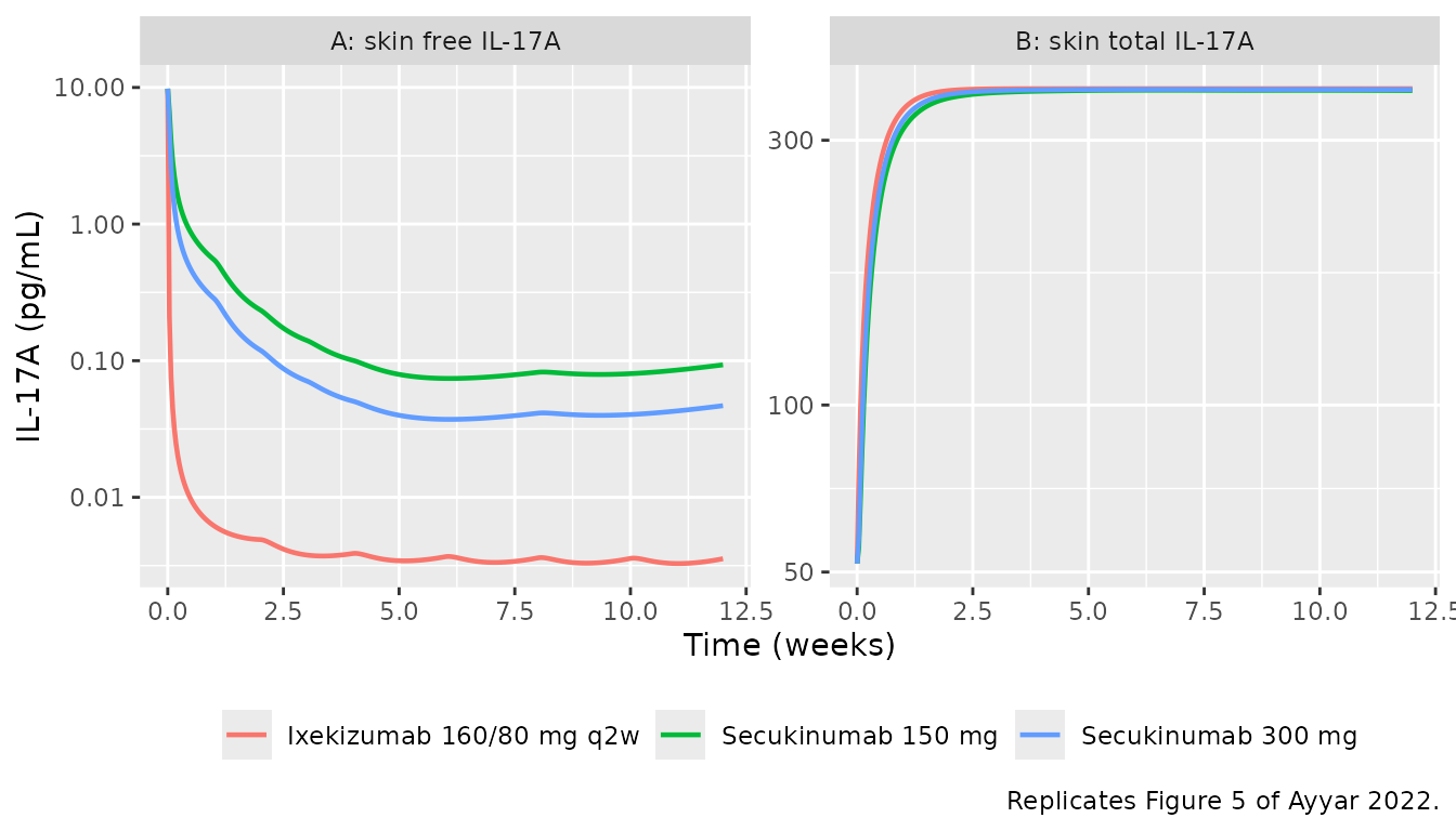
In Figure 5A at week 8, free skin IL-17A is about 0.08 pg/mL for secukinumab 150 mg, 0.04 pg/mL for 300 mg and 0.0035 pg/mL for ixekizumab. In Figure 5B, total skin IL-17A plateaus within 2-3 weeks, at about 360 / 50 times its baseline. These ratios do not depend on any unit conversion, so they are checked here.
wk8 <- sims12 |>
  dplyr::filter(time == 56) |>
  dplyr::select(regimen, Cfree_target_skin, Ctotal_target_skin)
wk8
#>                    regimen Cfree_target_skin Ctotal_target_skin
#> 1       Secukinumab 300 mg      0.0011797405           2.002353
#> 2       Secukinumab 150 mg      0.0023499601           1.995349
#> 3 Ixekizumab 160/80 mg q2w      0.0001029483           2.008799
free_300 <- wk8$Cfree_target_skin[wk8$regimen == "Secukinumab 300 mg"]
ratio_150 <- wk8$Cfree_target_skin[wk8$regimen == "Secukinumab 150 mg"] / free_300
ratio_ixe <- wk8$Cfree_target_skin[wk8$regimen == "Ixekizumab 160/80 mg q2w"] / free_300
c(ratio_150 = ratio_150, ratio_ixe = ratio_ixe)
#>  ratio_150  ratio_ixe
#> 1.99192969 0.08726354
stopifnot(
  abs(log(ratio_150 / (0.08 / 0.04))) < log(1.3),
  abs(log(ratio_ixe / (0.0035 / 0.04))) < log(1.3),
  all(abs(wk8$Ctotal_target_skin / 0.28 / (360 / 50) - 1) < 0.15)
)
Figure 3: secukinumab serum PK, serum total IL-17A and skin PK
The SC panels need no body weight, so they are reproduced here: the regimen-finding study (Figure 3B), the low dose-ranging study (Figure 3C), the Phase 3 regimens (Figure 3E) and the biodistribution study (Figure 3F). The IV panels (Figure 3A, 3D) are dosed in mg/kg, and the paper does not state the body weight it used, so they are not reproduced.
g40 <- seq(0, 280, by = 1)
fig3 <- dplyr::bind_rows(
  solve_regimen(mod_sec, 150, 0, g40, "B: 150 mg SC at wk 0"),
  solve_regimen(mod_sec, rep(150, 3), c(0, 28, 56), g40, "B: 150 mg SC at wk 0,4,8"),
  solve_regimen(mod_sec, rep(150, 4), c(0, 7, 14, 28), g40, "B: 150 mg SC at wk 0,1,2,4"),
  solve_regimen(mod_sec, rep(25, 3), c(0, 28, 56), g40, "C: 25 mg at wk 0,4,8"),
  solve_regimen(mod_sec, rep(75, 3), c(0, 28, 56), g40, "C: 75 mg at wk 0,4,8"),
  solve_regimen(mod_sec, rep(150, 3), c(0, 28, 56), g40, "C: 150 mg at wk 0,4,8")
) |>
  dplyr::mutate(panel = substr(regimen, 1, 1), Cc_ugmL = pM_to_ugmL(Cc))
ggplot(fig3, aes(time / 7, Cc_ugmL, colour = regimen)) +
  geom_line() +
  facet_wrap(~panel, ncol = 2) +
  scale_y_log10(limits = c(0.01, 100)) +
  labs(
    x = "Time (weeks)", y = "Serum secukinumab (ug/mL)", colour = NULL,
    caption = "Replicates Figure 3B-C of Ayyar 2022."
  ) +
  theme(legend.position = "bottom") +
  guides(colour = guide_legend(ncol = 2))
#> Warning in scale_y_log10(limits = c(0.01, 100)): log-10 transformation
#> introduced infinite values.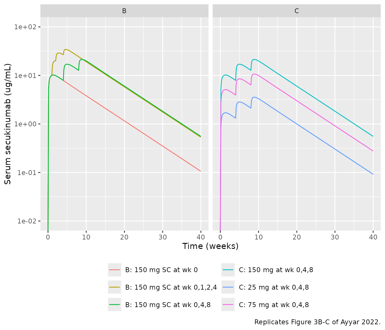
sec_p3_days <- c(0, 7, 14, 21, seq(28, 364, by = 28))
g56 <- seq(0, 392, by = 1)
fig3e <- dplyr::bind_rows(
  solve_regimen(mod_sec, rep(150, length(sec_p3_days)), sec_p3_days, g56, "150 mg SC at wk 0,1,2,3,4; then q4w"),
  solve_regimen(mod_sec, rep(300, length(sec_p3_days)), sec_p3_days, g56, "300 mg SC at wk 0,1,2,3,4; then q4w")
)
fig3e |>
  dplyr::transmute(
    time, regimen,
    `Serum secukinumab (ug/mL)` = pM_to_ugmL(Cc),
    `Serum total IL-17A (pg/mL)` = Ctotal_target * il17_total_pgmL_per_pM
  ) |>
  tidyr::pivot_longer(-c(time, regimen)) |>
  ggplot(aes(time / 7, value, colour = regimen)) +
  geom_line() +
  facet_wrap(~name, scales = "free_y") +
  scale_y_log10() +
  labs(x = "Time (weeks)", y = NULL, colour = NULL, caption = "Replicates Figure 3E of Ayyar 2022.") +
  theme(legend.position = "bottom")
#> Warning in scale_y_log10(): log-10 transformation introduced infinite values.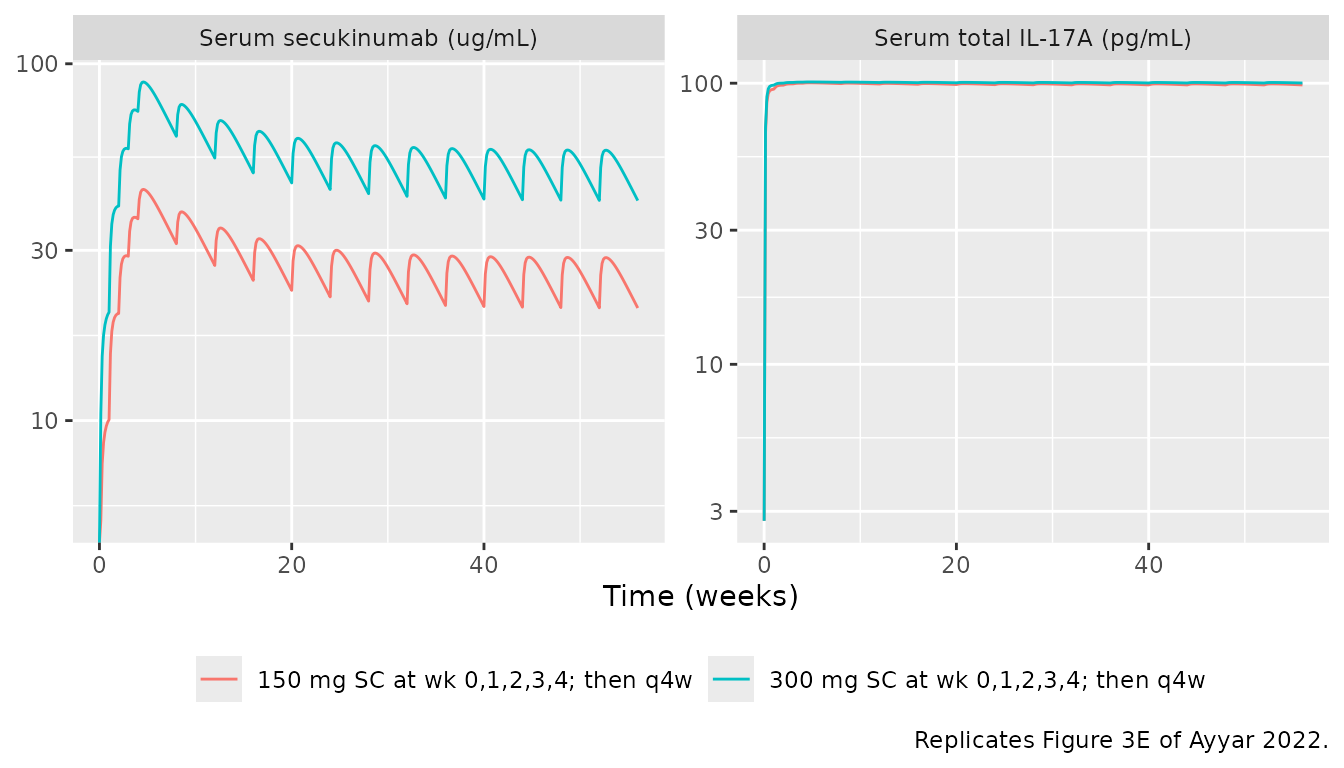
In Figure 3E, the 300 mg troughs run at about 30-40 ug/mL and the 150 mg troughs at about 15-20 ug/mL, and serum total IL-17A rises from about 2.8 to about 100 pg/mL. The conversion-free check is the IL-17A plateau/baseline ratio (about 100 / 2.8) and the trough concentrations:
e_chk <- fig3e |>
  dplyr::filter(time == 364) |>
  dplyr::mutate(trough_ugmL = pM_to_ugmL(Cc), il17_ratio = Ctotal_target / 0.015)
e_chk[, c("regimen", "trough_ugmL", "il17_ratio")]
#>                               regimen trough_ugmL il17_ratio
#> 1 150 mg SC at wk 0,1,2,3,4; then q4w    20.69945   35.52510
#> 2 300 mg SC at wk 0,1,2,3,4; then q4w    41.40166   36.09977
stopifnot(
  all(abs(e_chk$il17_ratio / (100 / 2.8) - 1) < 0.15),
  e_chk$trough_ugmL[1] > 12, e_chk$trough_ugmL[1] < 25,
  e_chk$trough_ugmL[2] > 25, e_chk$trough_ugmL[2] < 50
)
fig3f <- solve_regimen(mod_sec, 300, 0, seq(0, 56, by = 0.25), "300 mg SC")
fig3f |>
  dplyr::transmute(time, `Serum` = pM_to_ugmL(Cc), `Skin ISF` = pM_to_ugmL(Cis_skin)) |>
  tidyr::pivot_longer(-time) |>
  ggplot(aes(time / 7, value, colour = name)) +
  geom_line() +
  scale_y_log10(limits = c(0.1, 100)) +
  labs(x = "Time (weeks)", y = "Secukinumab (ug/mL)", colour = NULL, caption = "Replicates Figure 3F of Ayyar 2022.")
#> Warning in scale_y_log10(limits = c(0.1, 100)): log-10 transformation
#> introduced infinite values.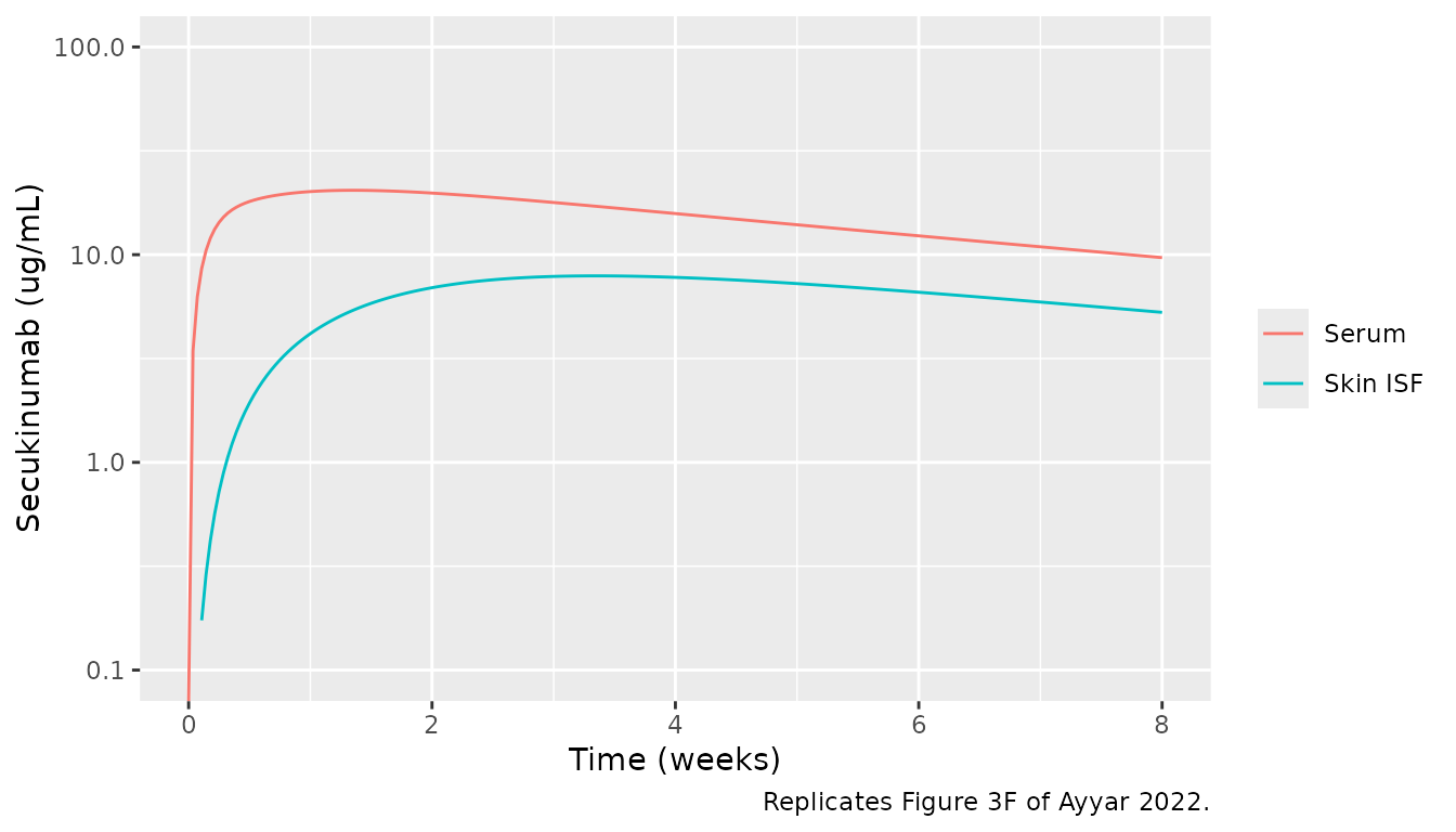
Figure 3F shows serum secukinumab at about 20 ug/mL over weeks 1-2. Skin rises to about 8 ug/mL by week 3 and then declines in parallel with serum.
Figure 4: ixekizumab serum PK
ixe_q2w <- c(0, seq(14, 84, by = 14))
ixe_q4w <- c(0, seq(28, 84, by = 28))
g12 <- seq(0, 112, by = 0.5)
fig4 <- dplyr::bind_rows(
  solve_regimen(mod_ixe, c(160, rep(80, length(ixe_q2w) - 1)), ixe_q2w, g12, "160 mg, then 80 mg q2w"),
  solve_regimen(mod_ixe, c(160, rep(80, length(ixe_q4w) - 1)), ixe_q4w, g12, "160 mg, then 80 mg q4w"),
  solve_regimen(mod_ixe, rep(150, 3), c(0, 14, 28), g12, "150 mg SC at wk 0,2,4")
)
ggplot(fig4, aes(time / 7, pM_to_ugmL(Cc), colour = regimen)) +
  geom_line() +
  scale_y_log10() +
  labs(x = "Time (weeks)", y = "Serum ixekizumab (ug/mL)", colour = NULL, caption = "Replicates Figure 4 of Ayyar 2022 (regimens of Table 1).") +
  theme(legend.position = "bottom")
#> Warning in scale_y_log10(): log-10 transformation introduced infinite values.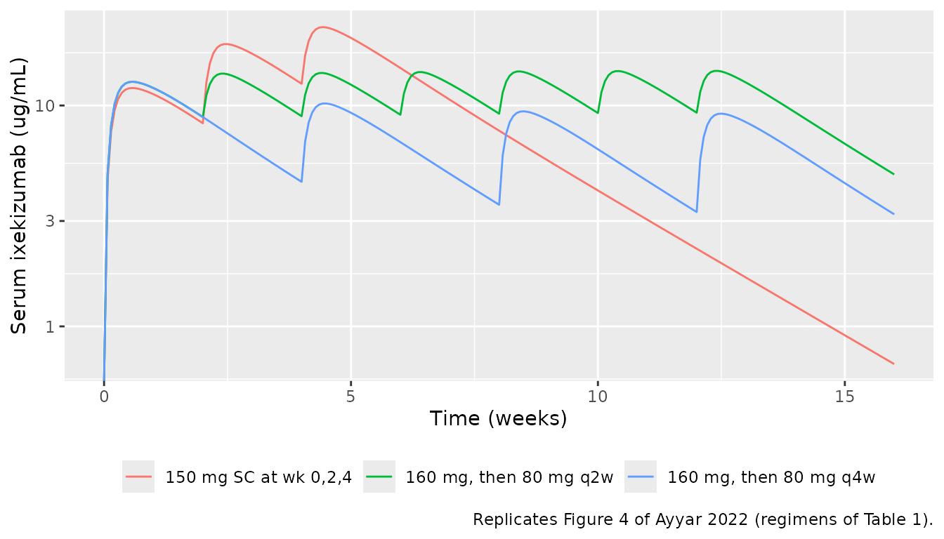
Figure 6: TE-based MBMA
The TE-MBMA trend line is shared by the two drugs. Here it is evaluated directly from the model parameters over the plotted range of free skin IL-17A, and the three approved regimens are placed on it at their simulated TE.
p <- as.list(mod_sec$theta)
te_curve <- function(x, e0, emax, ec50, h) e0 + x^h * (emax - e0) / (x^h + ec50^h)
xx <- 10^seq(-1, log10(25), length.out = 200)
curves <- dplyr::bind_rows(
  data.frame(endpoint = "PASI75", x = xx, y = te_curve(xx, p$e0_pasi75, p$emax_pasi75, exp(p$lec50_pasi75), p$hill_pasi75)),
  data.frame(endpoint = "PASI90", x = xx, y = te_curve(xx, p$e0_pasi90, p$emax_pasi90, exp(p$lec50_pasi90), p$hill_pasi90))
)
pts <- sims12 |>
  dplyr::filter(time == 84) |>
  dplyr::select(regimen, x = free_target_skin_avg_pct, PASI75 = prob_pasi75_pbo_adj, PASI90 = prob_pasi90_pbo_adj) |>
  tidyr::pivot_longer(c(PASI75, PASI90), names_to = "endpoint", values_to = "y") |>
  dplyr::mutate(y = 100 * y)
ggplot(curves, aes(x, y)) +
  geom_line(colour = "darkred", linewidth = 1) +
  geom_point(data = pts, aes(colour = regimen), size = 3) +
  facet_wrap(~endpoint) +
  scale_x_log10() +
  coord_cartesian(ylim = c(0, 100)) +
  labs(
    x = "Average predicted free IL-17A in skin (% baseline)",
    y = "Placebo-adjusted response (%)", colour = NULL,
    caption = "Replicates the trend lines of Figure 6 of Ayyar 2022."
  ) +
  theme(legend.position = "bottom")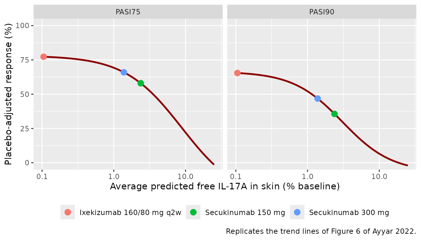
Figure 6 shows the trend line at about 77% (PASI75) and 66% (PASI90) near 0.1% free IL-17A, and crossing 0 at about 23% (PASI75) and 18% (PASI90). The digitised parameters reproduce this:
chk6 <- c(
  p75_at_0.1 = te_curve(0.1, p$e0_pasi75, p$emax_pasi75, exp(p$lec50_pasi75), p$hill_pasi75),
  p90_at_0.1 = te_curve(0.1, p$e0_pasi90, p$emax_pasi90, exp(p$lec50_pasi90), p$hill_pasi90),
  p75_at_23 = te_curve(23, p$e0_pasi75, p$emax_pasi75, exp(p$lec50_pasi75), p$hill_pasi75),
  p90_at_18 = te_curve(18, p$e0_pasi90, p$emax_pasi90, exp(p$lec50_pasi90), p$hill_pasi90)
)
round(chk6, 1)
#> p75_at_0.1 p90_at_0.1  p75_at_23  p90_at_18
#>       77.3       65.5        0.4        0.2
stopifnot(
  abs(chk6[["p75_at_0.1"]] - 77) < 2, abs(chk6[["p90_at_0.1"]] - 66) < 2,
  abs(chk6[["p75_at_23"]]) < 3, abs(chk6[["p90_at_18"]]) < 3
)
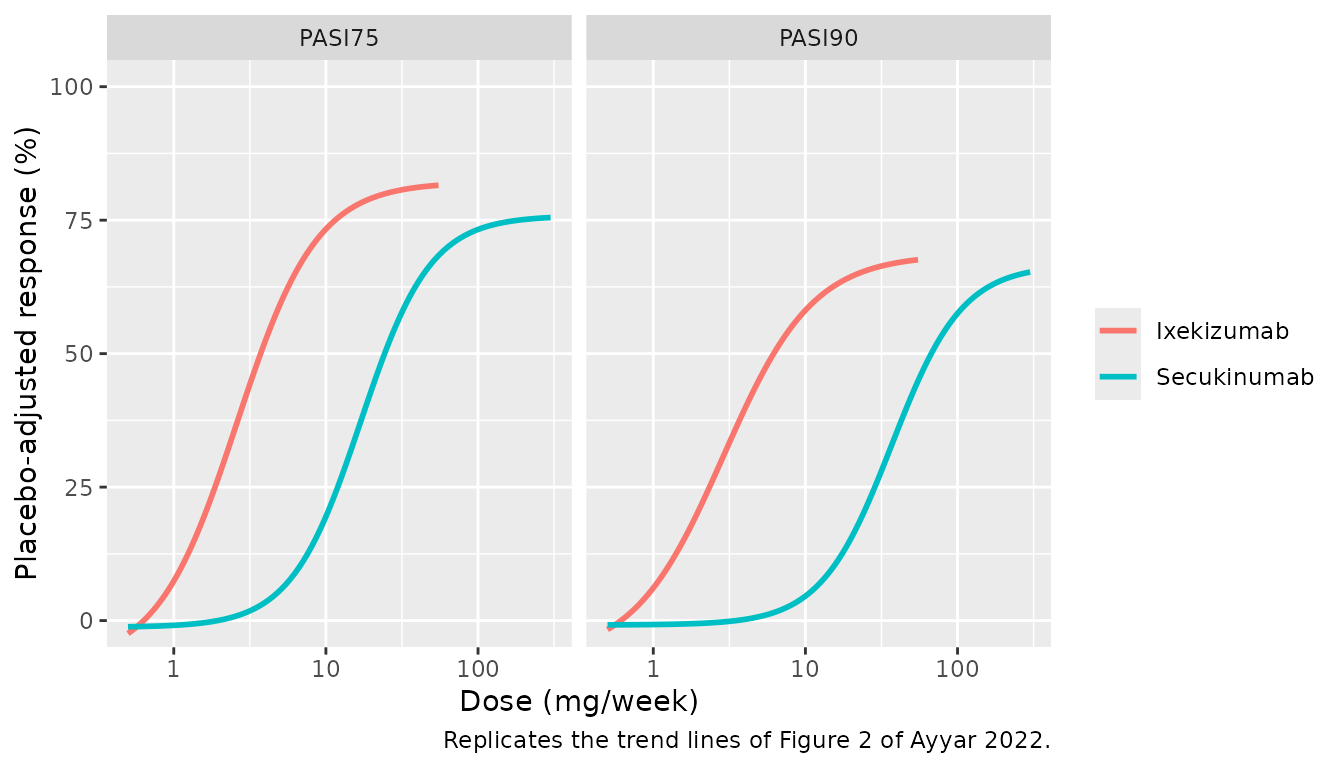
Figure 2: dose-based MBMA
The dose-based models are purely algebraic. They take the arm’s
average weekly dose over 12 weeks as the covariate
DOSE_<drug>_MGWK and need no dose events.
dose_grid <- function(drug, xmax) {
  x <- 10^seq(log10(0.5), log10(xmax), length.out = 100)
  d <- data.frame(id = seq_along(x), time = 0, evid = 0L, amt = 0, x = x)
  if (drug == "Secukinumab") d$DOSE_SECUKINUMAB_MGWK <- x else d$DOSE_IXEKIZUMAB_MGWK <- x
  d
}
fig2 <- dplyr::bind_rows(
  rxode2::rxSolve(mbma_sec, dose_grid("Secukinumab", 300), keep = "x", returnType = "data.frame") |> dplyr::mutate(drug = "Secukinumab"),
  rxode2::rxSolve(mbma_ixe, dose_grid("Ixekizumab", 55), keep = "x", returnType = "data.frame") |> dplyr::mutate(drug = "Ixekizumab")
) |>
  dplyr::select(drug, x, PASI75 = prob_pasi75_pbo_adj, PASI90 = prob_pasi90_pbo_adj) |>
  tidyr::pivot_longer(c(PASI75, PASI90), names_to = "endpoint", values_to = "y")
#> Warning: multi-subject simulation without without 'omega'
#> Warning: multi-subject simulation without without 'omega'
ggplot(fig2, aes(x, 100 * y, colour = drug)) +
  geom_line(linewidth = 1) +
  facet_wrap(~endpoint) +
  scale_x_log10() +
  coord_cartesian(ylim = c(0, 100)) +
  labs(
    x = "Dose (mg/week)", y = "Placebo-adjusted response (%)", colour = NULL,
    caption = "Replicates the trend lines of Figure 2 of Ayyar 2022."
  )
# Figure 2 trend lines read at 10 and 100 mg/week (secukinumab) and at 2 and
# 20 mg/week (ixekizumab).
f2 <- fig2 |>
  dplyr::group_by(drug, endpoint) |>
  dplyr::summarise(
    lo = approx(log(x), 100 * y, xout = log(ifelse(drug[1] == "Secukinumab", 10, 2)))$y,
    hi = approx(log(x), 100 * y, xout = log(ifelse(drug[1] == "Secukinumab", 100, 20)))$y,
    .groups = "drop"
  )
knitr::kable(f2, digits = 1)| drug | endpoint | lo | hi |
|---|---|---|---|
| Ixekizumab | PASI75 | 27.4 | 79.1 |
| Ixekizumab | PASI90 | 20.8 | 64.4 |
| Secukinumab | PASI75 | 19.5 | 73.3 |
| Secukinumab | PASI90 | 4.6 | 57.5 |
# Digitised Figure 2 trend-line values at the same doses
fig2_read <- c(
  "Ixekizumab.PASI75" = 25.5, "Ixekizumab.PASI90" = 20.2,
  "Secukinumab.PASI75" = 19.8, "Secukinumab.PASI90" = 3.8
)
fig2_read_hi <- c(
  "Ixekizumab.PASI75" = 78.9, "Ixekizumab.PASI90" = 64.6,
  "Secukinumab.PASI75" = 72.7, "Secukinumab.PASI90" = 56.8
)
key <- paste(f2$drug, f2$endpoint, sep = ".")
stopifnot(
  all(abs(f2$lo - fig2_read[key]) < 3),
  all(abs(f2$hi - fig2_read_hi[key]) < 3)
)
Read off Figure 2, the secukinumab PASI75 line is at about 20% at 10 mg/week and 73% at 100 mg/week. The ixekizumab line is at about 26% at 2 mg/week and 79% at 20 mg/week.
The Methods define the dose regressor as the total dose given over the first 12 weeks divided by 12 weeks. The trial arms in Figure 2 are plotted below that definition. The Phase 3 secukinumab 150 mg and 300 mg arms sit at about 55 and 110 mg/week rather than 900 / 12 = 75 and 1800 / 12 = 150. The Phase 3 ixekizumab 80 mg q4w and q2w arms sit at about 22 and 38 mg/week rather than 320 / 12 = 27 and 560 / 12 = 47. The paper does not explain the difference. The trend lines are reproduced as plotted, so a user who computes the regressor from the stated definition will place a regimen to the right of where the paper plotted it.
PKNCA: single-dose serum PK
The paper reports no NCA. The table below gives the single-dose serum NCA of the typical-value model for each drug’s SC doses, for reference. The model clearances (0.154 and 0.379 L/day) are close to the popPK total clearances the paper cites (0.19 and 0.29 L/day).
nca_days <- seq(0, 168, by = 1)
nca_sim <- dplyr::bind_rows(
  solve_regimen(mod_sec, 150, 0, nca_days, "Secukinumab 150 mg SC"),
  solve_regimen(mod_sec, 300, 0, nca_days, "Secukinumab 300 mg SC"),
  solve_regimen(mod_ixe, 80, 0, nca_days, "Ixekizumab 80 mg SC"),
  solve_regimen(mod_ixe, 160, 0, nca_days, "Ixekizumab 160 mg SC")
) |>
  dplyr::mutate(id = as.integer(factor(regimen)), Cc = pM_to_ugmL(Cc)) |>
  dplyr::filter(!is.na(Cc)) |>
  dplyr::select(id, time, Cc, treatment = regimen)
dose_df <- nca_sim |>
  dplyr::distinct(id, treatment) |>
  dplyr::mutate(time = 0, dose = as.numeric(sub(".* ([0-9]+) mg SC", "\\1", treatment)))

conc_obj <- PKNCA::PKNCAconc(nca_sim, Cc ~ time | treatment + id)
dose_obj <- PKNCA::PKNCAdose(dose_df, dose ~ time | treatment + id)
intervals <- data.frame(start = 0, end = Inf, cmax = TRUE, tmax = TRUE, aucinf.obs = TRUE, half.life = TRUE)
nca_res <- PKNCA::pk.nca(PKNCA::PKNCAdata(conc_obj, dose_obj, intervals = intervals))
nca_tab <- as.data.frame(nca_res$result) |>
  dplyr::filter(PPTESTCD %in% c("cmax", "tmax", "aucinf.obs", "half.life")) |>
  dplyr::select(treatment, PPTESTCD, PPORRES) |>
  tidyr::pivot_wider(names_from = PPTESTCD, values_from = PPORRES) |>
  dplyr::rename(
    Regimen = treatment,
    `Cmax (ug/mL)` = cmax,
    `Tmax (day)` = tmax,
    `AUC0-inf (ug*day/mL)` = aucinf.obs,
    `t1/2 (day)` = half.life
  )
knitr::kable(nca_tab, digits = 2)| Regimen | Cmax (ug/mL) | Tmax (day) | t1/2 (day) | AUC0-inf (ug*day/mL) |
|---|---|---|---|---|
| Ixekizumab 160 mg SC | 12.80 | 4 | 15.89 | 340.74 |
| Ixekizumab 80 mg SC | 6.40 | 4 | 15.80 | 170.29 |
| Secukinumab 150 mg SC | 10.20 | 9 | 40.58 | 708.87 |
| Secukinumab 300 mg SC | 20.41 | 9 | 40.60 | 1418.13 |
Assumptions and deviations
-
Molar units and molecular weight. The models take
doses in pmol and report pM. The paper does not state the antibody
molecular weight; this vignette uses a nominal 150 kDa
(
1 mg = 6667 pmol). With it, the printed TE values (98.6% and 99.9%) are reproduced to the printed precision, and a +/- 10 kDa change moves them by less than 0.1 percentage point. - IL-17A pg/mL axes. The paper’s figures report IL-17A in pg/mL but do not state the conversion from the model’s pM, and the panels are not consistent. The free IL-17A of Figure 5A corresponds to about 35 pg/mL per pM, the mass of the IL-17A homodimer. The total IL-17A of Figures 3E and 5B corresponds to about 185 pg/mL per pM, the mass of an antibody-IL-17A complex. The models reproduce the paper’s pM values (Table 2 baselines). The two factors are used here only for display, and the checks above use conversion-free ratios. A user comparing total IL-17A with assay data in pg/mL of IL-17A should note that the fitted serum total IL-17A data appear to have been converted with the complex mass.
-
Ixekizumab parameters fixed to secukinumab. Table 2
footnote b states that the ixekizumab serum complex elimination rate
kintand skin reflection coefficientsigma_skinwere “assumed to be the same as for secukinumab”. They are coded asfixed()in the ixekizumab model. - Leaky-tissue volume. The control stream fixes V2 = 4.368 L; Table 2 prints the rounded 4.37 L. The unrounded value is used.
-
Lymph equation. DataSheet1 Eq. 6 writes the lymph
inflows with the vascular reflection coefficients
(1 - sigma_sk),(1 - sigma_1)and(1 - sigma_2). The tissue equations (Eq. 3-5) and the control stream use the lymphatic coefficient(1 - sigma_L)for the same flows. The control stream form is used because it conserves mass between tissue and lymph. - IIV. The Methods state that IIV was not considered and the variance-covariance matrix was fixed to zero. The supplementary control stream nevertheless carries two estimable omegas (CL and Vp) with initial value 0.1. The models follow the Methods and have no random effects.
-
Residual error. Each fitted output had an additive
error on log concentrations, which the paper calls proportional. The
magnitudes are not reported, so they are
lnorm()with standard deviationfixed(0). -
QE free-drug formula. The printed
0.5 * (a + sqrt(a^2 + 4 KD C)), witha = C - KD - Rtot, loses precision at low drug concentration. The models use the algebraically identical2 KD C / (sqrt(a^2 + 4 KD C) - a)whena < 0. -
SC bioavailability. The control stream multiplies
the absorption rate by F. The models put F on the depot dose instead
(
f(depot)), which gives the same plasma input. -
MBMA parameters digitised. None of the MBMA
parameters are printed. They were digitised from the Figure 2 and Figure
6 trend lines and refitted. The dose-based E0 values are slightly
negative because the plotted lines start at 0.5 mg/week and do not
identify E0. Below 3 mg/week the ixekizumab line is a polyline through a
coarse simulation grid, so only its vertices were used. The TE-based
PASI75
emax(-26.9) lies below zero because the authors’ fit reaches 0% response at about 23% free IL-17A without leveling off. Use the MBMAs only over the plotted ranges. - IV panels not reproduced. Figures 3A and 3D use mg/kg IV doses, and the paper gives no body weight to convert them.