Model and source
- Citation: Onita T, Sano Y, Ikawa K, Ishihara N, Tamaki H, Yano T. Population pharmacokinetic analysis and pharmacodynamic evaluation of sulbactam in pediatric patients: dosing suggestions for Acinetobacter baumannii infections. J Pediatric Infect Dis Soc. 2025;14(5):piaf043. doi:10.1093/jpids/piaf043. All structural, covariate, interindividual-variability and residual-error estimates are from Supplementary Table S1; the free fraction and the 60% fT > MIC target are from the Methods section ‘Estimation of the PK/PD Parameter’.
- Description: Two-compartment population PK model for intravenous sulbactam in 122 pediatric patients (4 weeks to 16.4 years), built by pooled analysis of 690 plasma concentrations digitised from 23 published pediatric sulbactam PK studies identified by a MEDLINE search (Onita 2025). Clearance carries two separate allometric power terms, both with a fixed exponent of 0.75: one on body weight normalised to the cohort median 22.45 kg, and one on age normalised to the cohort median 8 years; the age term is the novel feature of this model and drives an order-of-magnitude lower weight- normalised clearance in infants than in adolescents. Central volume is linear in body weight (exponent 1); intercompartmental clearance and peripheral volume carry no covariates. Exponential interindividual variability is estimated on all four structural parameters and residual error is proportional. The model also returns the unbound plasma concentration Cu (71.2% free fraction), which indexes the paper’s 60% fT > MIC probability-of-target-attainment analysis against Acinetobacter baumannii.
- Article: https://doi.org/10.1093/jpids/piaf043
- Supplementary Table S1 (all parameter estimates) and Supplementary Figure S1 (goodness-of-fit plots) are distributed with the open-access article (PMC12123189).
Onita and colleagues pooled individual plasma concentration-time data from 23 previously published pediatric sulbactam studies identified by a MEDLINE search and fitted a single two-compartment population PK model in NONMEM 7 (ADVAN3, FOCE). The distinguishing feature of the model is that age enters clearance as a second allometric term alongside body weight, which the authors highlight as novel for sulbactam. The model was then used to evaluate the probability of attaining the bactericidal target of 60% fT > MIC against Acinetobacter baumannii.
Note that this is not a systematic review that tabulates other authors’ models: the literature search supplied raw concentration-time observations, and the popPK model fitted to them is original to this paper.
Population
The model was built from 122 pediatric patients contributing 690 plasma samples across 23 pooled publications (Table 1 of Onita 2025). Ages ranged from 0.083 to 16.42 years (mean 7.5, SD 4.0; median 8) and body weights from 4 to 77 kg (mean 24.7, SD 13.4; median 22.45). Sex was reported as 69 male, 49 female and 4 not applicable, i.e. 40.2% female. The three age strata used for the dosing analysis were infants (4 weeks to 11 months, n = 10, 8.2%), children (1-6 years, n = 44, 36.1%) and pediatrics (7-16 years, n = 68, 55.7%). Doses ranged from 4.9 to 41.7 mg/kg given as an intravenous bolus or a 0.5-hour or 1-hour infusion.
Underlying disease, treatment indication and renal function (serum creatinine, blood urea nitrogen) were not available in the pooled source publications; the authors identify this as the study’s principal limitation. Concentrations were measured by bioassay in 20 of the 23 pooled studies and by an unclear method in the remaining 3.
The same information is available programmatically:
str(readModelDb("Onita_2025_sulbactam")()$population)
#> List of 16
#>  $ species       : chr "human"
#>  $ n_subjects    : int 122
#>  $ n_studies     : int 23
#>  $ n_observations: int 690
#>  $ age_range     : chr "0.083-16.42 years"
#>  $ age_median    : chr "8 years"
#>  $ age_mean      : chr "7.5 years (SD 4.0)"
#>  $ weight_range  : chr "4-77 kg"
#>  $ weight_median : chr "22.45 kg"
#>  $ weight_mean   : chr "24.7 kg (SD 13.4)"
#>  $ sex_female_pct: num 40.2
#>  $ age_strata    : Named int [1:3] 10 44 68
#>   ..- attr(*, "names")= chr [1:3] "infant (4 weeks to 11 months)" "child (1-6 years)" "pediatric (7-16 years)"
#>  $ disease_state : chr "Not reported. The pooled source publications did not record underlying disease, treatment indication, or renal "| __truncated__
#>  $ dose_range    : chr "4.9-41.7 mg/kg IV, given as a bolus or a 0.5-hour or 1-hour infusion"
#>  $ regions       : chr "Not reported; source publications identified by MEDLINE search"
#>  $ notes         : chr "Baseline demographics are Table 1 of Onita 2025 (N = 122; sex male/female/not-applicable 69:49:4, so the female"| __truncated__
Source trace
Every ini() entry in
inst/modeldb/specificDrugs/Onita_2025_sulbactam.R carries
an in-file comment naming its origin. They are collected here for
review.
| Equation / parameter | Value | Source location |
|---|---|---|
d/dt(central), d/dt(peripheral1)
|
n/a | Methods, “Population PK Modeling”:
dXc/dt = -(CL/Vc + Q/Vc) x Xc + Q x Xp/Vp;
dXp/dt = Q x Xc/Vc - Q x Xp/Vp
|
| CL covariate equation | thetaCL x (BWT/22.45)^0.75 x (AGE/8)^0.75 |
Table S1, “Fix effects parameter” |
| Vc covariate equation | thetaVcentral x (BWT/22.45) |
Table S1, “Fix effects parameter” |
lcl |
7.65 L/h | Table S1: thetaCL(L/h) 7.65 (5.84) 6.58-8.47
|
lvc |
4.75 L | Table S1: thetaVcentral (L) 4.75 (7.5) 4.13-5.79
|
lq |
3.03 L/h | Table S1: Q (L/h) = thetaQ 3.03 (11.1) 2.19-3.76
|
lvp |
4.88 L | Table S1:
Vperipheral (L) = thetaVperipheral 4.88 (10.4) 3.88-6.91
|
e_wt_cl |
0.75 (fixed) | Table S1 equation (BWT/22.45)^0.75; Methods: “A
standard allometric scaling exponent of 0.75 was included” |
e_age_cl |
0.75 (fixed) | Table S1 equation (AGE/8)^0.75
|
e_wt_vc |
1 (fixed) | Table S1 equation
Vcentral (L) = thetaVcentral x (BWT/22.45), printed with no
exponent |
wtref |
22.45 kg (fixed) | Table S1 footnote a: “Median as body weight in 122 subjects” |
ageref |
8 years (fixed) | Table S1 footnote b: “Median as age in 122 subjects” |
etalcl |
0.229 (variance) | Table S1: etaCL 0.229 (25.1) 0.134-0.388
|
etalvc |
0.223 (variance) | Table S1: etaVcentral 0.223 (43.1) 0.0430-0.431
|
etalq |
0.430 (variance) | Table S1: etaQ 0.430 (28.3) 0.184-0.690
|
etalvp |
0.504 (variance) | Table S1: etaVperipheral 0.504 (27.0) 0.275-0.964
|
propSd |
0.2644 = sqrt(0.0699) | Table S1: epsilon 0.0699 (19.8) 0.0421-0.102
|
fu |
0.712 (fixed) | Methods, “Estimation of the PK/PD Parameter”: “a value of 71.2% nonprotein-binding rate (the free fraction f) of sulbactam was used” |
| 60% fT > MIC target | n/a | Methods, “Estimation of the PK/PD Parameter” |
| CLSI breakpoints 4 / 8 / 16 ug/mL | n/a | Methods, “Microbiological Data” |
Variance versus standard deviation
The interindividual and residual entries in Table S1 are variances, not standard deviations or coefficients of variation. Two independent statements in the source fix this:
- The Methods define the IIV model as
theta_i = theta x exp(eta_i)where eta is “normally distributed with a mean of 0 and variance of omega^2”. - The Table S1 footnotes repeat, for both symbols, “normally distributed with a mean of zero and variance”.
The eta values are therefore passed to ini() unsquared,
and the proportional residual standard deviation is
sqrt(0.0699) = 0.2644 (26.4%).
Structural identity check against the published typical values
The Discussion states the model’s typical values in weight-normalised form:
“these reported values are similar to ours (CL: 0.31 (L/h/kg), V (Vc + Vp): 0.39 (L/kg) as mean body weight 24.7 kg)”.
These two numbers are an answer key for the whole parameterisation,
because they hold only if the Table S1 estimates are the values at the
reference covariates (WT = 22.45 kg, AGE = 8
years), where both allometric multipliers equal 1:
theta <- c(cl = 7.65, vc = 4.75, q = 3.03, vp = 4.88)
mean_wt <- 24.7  # Table 1 mean body weight

data.frame(
  Quantity = c("CL (L/h/kg)", "V = Vc + Vp (L/kg)"),
  Published = c(0.31, 0.39),
  Derived = round(c(theta[["cl"]], theta[["vc"]] + theta[["vp"]]) / mean_wt, 4)
)
#>             Quantity Published Derived
#> 1        CL (L/h/kg)      0.31  0.3097
#> 2 V = Vc + Vp (L/kg)      0.39  0.3899
Both reproduce the published figures exactly on rounding, confirming
that the Table S1 estimates are reference-covariate typical values and
that Vc and Vp are the two volumes summed in
the Discussion.
Non-compartmental validation against the published typical values
The same two numbers are now recovered through PKNCA rather than by arithmetic. A single intravenous bolus is given to a typical subject held at the reference covariates with all random effects zeroed, so the NCA-derived clearance and steady-state volume must return the structural parameters.
mod <- readModelDb("Onita_2025_sulbactam")
mod_typ <- rxode2::zeroRe(mod)
#> ℹ parameter labels from comments will be replaced by 'label()'

ref_dose <- 500  # mg; any dose reproduces CL and Vss for a linear model

ev_ref <-
  dplyr::bind_rows(
    data.frame(
      id = 1L, time = 0, amt = ref_dose, evid = 1L, cmt = "central"
    ),
    data.frame(
      id = 1L,
      time = c(seq(0, 2, by = 0.02), seq(2.1, 24, by = 0.1)),
      amt = NA_real_, evid = 0L, cmt = "central"
    )
  ) |>
  dplyr::mutate(WT = 22.45, AGE = 8) |>
  dplyr::arrange(.data$time, dplyr::desc(.data$evid))

# rxSolve() omits the `id` column for a single-subject solve, so it is
# restored explicitly before the data go to PKNCA (which groups on it).
sim_ref <-
  rxode2::rxSolve(mod_typ, ev_ref, returnType = "data.frame") |>
  dplyr::mutate(id = 1L, stratum = "Reference subject (22.45 kg, 8 years)")
#> ℹ omega/sigma items treated as zero: 'etalcl', 'etalvc', 'etalq', 'etalvp'

# Defensive time-zero record: PKNCA integrates from the interval start, so a
# missing t = 0 row triggers a per-subject "AUC range starting before the first
# measurement" warning.
sim_ref_nca <-
  sim_ref |>
  dplyr::filter(!is.na(.data$Cc)) |>
  dplyr::select("id", "time", "Cc", "stratum") |>
  dplyr::arrange(.data$id, .data$time) |>
  dplyr::distinct(.data$id, .data$time, .keep_all = TRUE)

stopifnot(any(sim_ref_nca$time == 0))
conc_ref <- PKNCA::PKNCAconc(
  sim_ref_nca, Cc ~ time | stratum + id,
  concu = "mg/L", timeu = "h"
)
dose_ref <- PKNCA::PKNCAdose(
  ev_ref |>
    dplyr::filter(.data$evid == 1L) |>
    dplyr::mutate(stratum = "Reference subject (22.45 kg, 8 years)") |>
    dplyr::select("id", "time", "amt", "stratum"),
  amt ~ time | stratum + id,
  doseu = "mg", route = "intravascular", duration = 0
)

intervals_ref <- data.frame(
  start = 0, end = Inf,
  cmax = TRUE, aucinf.obs = TRUE, half.life = TRUE,
  cl.obs = TRUE, vss.obs = TRUE
)

res_ref <- PKNCA::pk.nca(
  PKNCA::PKNCAdata(conc_ref, dose_ref, intervals = intervals_ref)
)
The reference values are the Table S1 structural parameters,
expressed as the quantities NCA estimates: total clearance
thetaCL, and steady-state volume
thetaVcentral + thetaVperipheral.
reference_ref <- data.frame(
  stratum = "Reference subject (22.45 kg, 8 years)",
  cl.obs = theta[["cl"]],
  vss.obs = theta[["vc"]] + theta[["vp"]]
)

tbl_ref <- nlmixr2lib::ncaComparisonTable(
  simulated = res_ref,
  reference = reference_ref,
  by = "stratum",
  params = c("cl.obs", "vss.obs"),
  units = c(cl.obs = "L/h", vss.obs = "L")
)
knitr::kable(tbl_ref, digits = 3)| NCA parameter | stratum | Reference | Simulated | % diff |
|---|---|---|---|---|
| CL/F (L/h) | Reference subject (22.45 kg, 8 years) | 7.65 | 7.65 | -0.0% |
| Vss/F (L) | Reference subject (22.45 kg, 8 years) | 9.63 | 9.63 | -0.0% |
attr(tbl_ref, "footnote")
#> NULL
Both parameters are recovered exactly, so the ODE system, the
covariate normalisation and the units (mg dose, L volume, giving mg/L,
which is numerically identical to the paper’s ug/mL) are all mutually
consistent. PKNCA’s default labels read CL/F and
Vss/F; sulbactam here is given intravenously, so F = 1 and
these are simply CL and Vss.
Virtual cohort
The individual data underlying the pooled analysis are not publicly available, and the paper does not publish the age or weight distribution within each of its three dosing strata – only the stratum boundaries and the overall cohort summary. The cohort below therefore samples age uniformly across each published stratum and assigns body weight from CDC/WHO median weight-for-age with a lognormal spread. This is an assumption; its consequences are quantified in the sensitivity analysis below.
set.seed(20250529)

# CDC/WHO median weight-for-age (50th percentile), used to give the virtual
# cohort a realistic weight for its sampled age.
wfa <- data.frame(
  age = c(0.083, 0.25, 0.5, 0.75, 1, 2, 3, 4, 5, 6, 7, 8, 9, 10,
          11, 12, 13, 14, 15, 16, 17),
  wt  = c(4.5, 6.4, 7.9, 8.9, 9.6, 12.2, 14.3, 16.3, 18.3, 20.5, 22.9, 25.3,
          28.1, 31.2, 34.7, 38.8, 43.4, 48.8, 53.8, 58.7, 61.8)
)
median_weight_for_age <- function(age) {
  stats::approx(wfa$age, wfa$wt, xout = age, rule = 2)$y
}

n_per_arm <- 200L  # cohort cap: never more than 200 participants per arm

strata <- data.frame(
  stratum = c("Infants (4 weeks to 11 months)",
              "Children (1-6 years)",
              "Pediatrics (7-16 years)"),
  age_lo = c(4 / 52, 1, 7),
  age_hi = c(11 / 12, 6, 16.42)
)

make_stratum <- function(stratum, age_lo, age_hi, id_offset) {
  age <- stats::runif(n_per_arm, age_lo, age_hi)
  data.frame(
    id = id_offset + seq_len(n_per_arm),
    stratum = stratum,
    AGE = age,
    WT = median_weight_for_age(age) * exp(stats::rnorm(n_per_arm, 0, 0.15))
  )
}

cohort <-
  dplyr::bind_rows(Map(
    make_stratum,
    strata$stratum, strata$age_lo, strata$age_hi,
    seq_len(nrow(strata)) * 1000L
  ))

stopifnot(nrow(cohort) == n_per_arm * nrow(strata), !anyDuplicated(cohort$id))
Because the cohort is synthetic, its fidelity to the published demographics is checked rather than assumed. Weighting the three strata by their published proportions (8.2% / 36.1% / 55.7%) should approximately recover the Table 1 overall summary.
strata_weight <- c(
  "Infants (4 weeks to 11 months)" = 0.082,
  "Children (1-6 years)" = 0.361,
  "Pediatrics (7-16 years)" = 0.557
)
set.seed(7)
# Resample the cohort in the published stratum proportions so a plain median
# reproduces the Table 1 whole-cohort statistics.
pooled <- cohort[
  sample(nrow(cohort), 5000L, replace = TRUE,
         prob = strata_weight[cohort$stratum]),
]

data.frame(
  Statistic = c("Median age (years)", "Median weight (kg)",
                "Min weight (kg)", "Max weight (kg)"),
  Published = c(8, 22.45, 4, 77),
  Simulated = round(c(
    stats::median(pooled$AGE), stats::median(pooled$WT),
    min(cohort$WT), max(cohort$WT)
  ), 2)
) |>
knitr::kable()| Statistic | Published | Simulated |
|---|---|---|
| Median age (years) | 8.00 | 7.75 |
| Median weight (kg) | 22.45 | 25.31 |
| Min weight (kg) | 4.00 | 3.91 |
| Max weight (kg) | 77.00 | 74.85 |
Concentration-time profiles by age stratum
Figure 1 of Onita 2025 is a prediction-corrected visual predictive
check against the pooled observed data. Those observations are not
redistributable, so the panel below instead shows the model-implied
10th, 50th and 90th percentiles – the same three percentiles the paper’s
VPC displays – over one steady-state dosing interval, using the
sim column so that residual error is included as it is in a
VPC.
tau <- 6      # q.i.d. dosing interval, hours
n_dose <- 20L  # doses to steady state
t_ss <- tau * (n_dose - 1L)

simulate_regimen <- function(cohort_df, mg_per_kg, infusion_h,
                             grid_by = 0.05, seed = 99L) {
  obs_times <- seq(t_ss, t_ss + tau, by = grid_by)
  ev <-
    dplyr::bind_rows(
      cohort_df |>
        dplyr::mutate(
          time = 0, amt = mg_per_kg * .data$WT, dur = infusion_h,
          evid = 1L, cmt = "central", ii = tau, addl = n_dose - 1L
        ),
      tidyr::expand_grid(
        cohort_df |> dplyr::select("id", "stratum", "AGE", "WT"),
        time = obs_times
      ) |>
        dplyr::mutate(
          amt = NA_real_, dur = NA_real_, evid = 0L, cmt = "central",
          ii = 0, addl = 0L
        )
    ) |>
    dplyr::arrange(.data$id, .data$time, dplyr::desc(.data$evid))

  set.seed(seed)  # common random numbers across regimens
  out <- rxode2::rxSolve(mod, ev, returnType = "data.frame",
                         keep = c("stratum", "AGE", "WT"))
  stopifnot(
    length(unique(out$id)) == nrow(cohort_df),
    nrow(out) == nrow(cohort_df) * length(obs_times)
  )
  out
}

sim_vpc <- simulate_regimen(cohort, mg_per_kg = 25, infusion_h = 0.5)
#> ℹ parameter labels from comments will be replaced by 'label()'

sim_vpc |>
  dplyr::mutate(time_in_tau = .data$time - t_ss) |>
  dplyr::group_by(.data$stratum, .data$time_in_tau) |>
  dplyr::summarise(
    p10 = stats::quantile(.data$sim, 0.10),
    p50 = stats::quantile(.data$sim, 0.50),
    p90 = stats::quantile(.data$sim, 0.90),
    .groups = "drop"
  ) |>
  ggplot2::ggplot(ggplot2::aes(x = time_in_tau)) +
  ggplot2::geom_ribbon(ggplot2::aes(ymin = p10, ymax = p90), alpha = 0.25,
                       fill = "steelblue") +
  ggplot2::geom_line(ggplot2::aes(y = p50), colour = "steelblue4") +
  ggplot2::facet_wrap(~stratum) +
  ggplot2::scale_y_log10() +
  ggplot2::labs(
    x = "Time within steady-state dosing interval (h)",
    y = "Sulbactam plasma concentration (mg/L)",
    title = "Model-implied 10th-90th percentile interval, 25 mg/kg q.i.d., 0.5-h infusion",
    caption = "Percentiles correspond to those displayed in Figure 1 of Onita 2025."
  )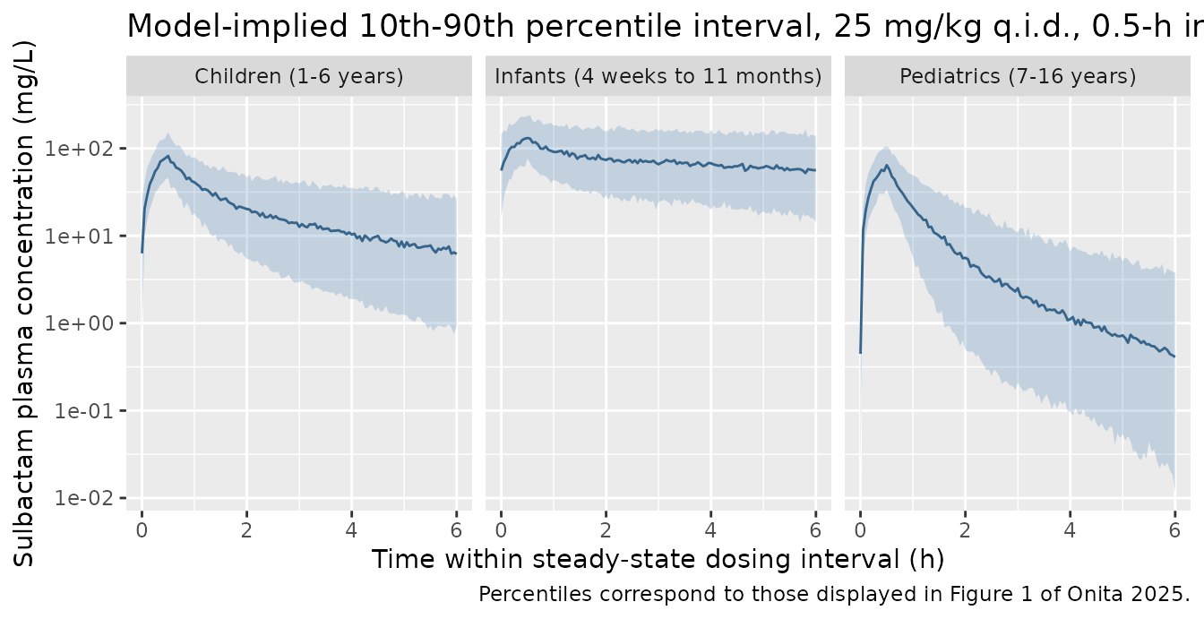
The infant panel sits an order of magnitude higher than the
adolescent panel at the end of the interval despite identical mg/kg
dosing. That separation is the direct consequence of the
(AGE/8)^0.75 term on clearance and is what drives the
dosing conclusions below.
Steady-state exposure by age stratum
nca_ss <- function(sim_df) {
  conc <-
    sim_df |>
    dplyr::filter(!is.na(.data$Cc)) |>
    dplyr::select("id", "time", "Cc", "stratum")

  dose_df <-
    sim_df |>
    dplyr::group_by(.data$id, .data$stratum) |>
    dplyr::summarise(WT = dplyr::first(.data$WT), .groups = "drop") |>
    dplyr::mutate(time = t_ss, amt = 25 * .data$WT)

  intervals <- data.frame(
    start = t_ss, end = t_ss + tau,
    cmax = TRUE, cmin = TRUE, tmax = TRUE, auclast = TRUE, cav = TRUE
  )

  PKNCA::pk.nca(PKNCA::PKNCAdata(
    PKNCA::PKNCAconc(conc, Cc ~ time | stratum + id,
                     concu = "mg/L", timeu = "h"),
    PKNCA::PKNCAdose(dose_df, amt ~ time | stratum + id,
                     doseu = "mg", route = "intravascular", duration = 0.5),
    intervals = intervals
  ))
}

res_ss <- nca_ss(sim_vpc)

as.data.frame(res_ss) |>
  dplyr::filter(.data$PPTESTCD %in% c("cmax", "cmin", "cav", "auclast")) |>
  dplyr::group_by(.data$stratum, .data$PPTESTCD) |>
  dplyr::summarise(median = stats::median(.data$PPORRES), .groups = "drop") |>
  tidyr::pivot_wider(names_from = "PPTESTCD", values_from = "median") |>
  dplyr::rename(
    "Age stratum" = "stratum",
    "Cmax,ss (mg/L)" = "cmax",
    "Cmin,ss (mg/L)" = "cmin",
    "Cav,ss (mg/L)" = "cav",
    "AUC0-tau (mg*h/L)" = "auclast"
  ) |>
  knitr::kable(digits = 2,
caption = "Median steady-state NCA parameters, 25 mg/kg q.i.d., 0.5-h infusion.")| Age stratum | AUC0-tau (mg*h/L) | Cav,ss (mg/L) | Cmax,ss (mg/L) | Cmin,ss (mg/L) |
|---|---|---|---|---|
| Children (1-6 years) | 135.23 | 22.54 | 85.01 | 6.73 |
| Infants (4 weeks to 11 months) | 473.24 | 78.87 | 136.79 | 58.39 |
| Pediatrics (7-16 years) | 58.27 | 9.71 | 62.63 | 0.48 |
Onita 2025 does not tabulate NCA parameters by stratum, so these are reported as model output rather than as a comparison against published values. The monotone decline in exposure from infants to adolescents is the expected consequence of the age term on clearance.
Replication of Table 2: PK/PD breakpoint MICs
This is the paper’s primary quantitative result. The bactericidal target is 60% fT > MIC computed on the unbound concentration (free fraction 0.712), and the PK/PD breakpoint is defined in the Table 2 footnote as “the largest MIC attaining more than 90% probabilities” of reaching that target.
The model returns Cu directly as the unbound
concentration. Following the paper’s own method – “The time point at
which the drug concentrations coincided with a specific MIC value was
determined, and T > MIC was calculated as the cumulative percentage
of 24 hours” – fT > MIC is computed by post-processing a
dense steady-state profile, not by an ODE accumulator.
mic_ladder <- c(0.06, 0.13, 0.25, 0.5, 1, 2, 4, 8, 16, 32, 64)

pta_for <- function(sim_df, mics = mic_ladder) {
  dplyr::bind_rows(lapply(mics, function(m) {
    # Per subject: fraction of the steady-state interval with unbound
    # concentration above the MIC. Then: fraction of subjects reaching 60%.
    sim_df |>
      dplyr::group_by(.data$stratum, .data$id) |>
      dplyr::summarise(ft_gt_mic = mean(.data$Cu > m), .groups = "drop") |>
      dplyr::group_by(.data$stratum) |>
      dplyr::summarise(
        mic = m,
        pta = 100 * mean(.data$ft_gt_mic >= 0.60),
        .groups = "drop"
      )
  }))
}

regimens <- tidyr::expand_grid(
  mg_per_kg = c(25, 50),
  infusion_h = c(0.5, 4)
)

pta_all <-
  dplyr::bind_rows(Map(
    function(mg_per_kg, infusion_h) {
      simulate_regimen(cohort, mg_per_kg, infusion_h) |>
        pta_for() |>
        dplyr::mutate(mg_per_kg = mg_per_kg, infusion_h = infusion_h)
    },
    regimens$mg_per_kg, regimens$infusion_h
  ))

breakpoints <-
  pta_all |>
  dplyr::group_by(.data$stratum, .data$mg_per_kg, .data$infusion_h) |>
  dplyr::summarise(
    breakpoint = if (any(.data$pta >= 90)) max(.data$mic[.data$pta >= 90]) else NA_real_,
    .groups = "drop"
  )
published_tbl2 <- tibble::tribble(
  ~stratum,                          ~mg_per_kg, ~infusion_h, ~published,
  "Infants (4 weeks to 11 months)",  25,         0.5,         16,
  "Infants (4 weeks to 11 months)",  50,         0.5,         32,
  "Infants (4 weeks to 11 months)",  25,         4,           16,
  "Infants (4 weeks to 11 months)",  50,         4,           32,
  "Children (1-6 years)",            25,         0.5,          1,
  "Children (1-6 years)",            50,         0.5,          2,
  "Children (1-6 years)",            25,         4,            8,
  "Children (1-6 years)",            50,         4,           16,
  "Pediatrics (7-16 years)",         25,         0.5,          0.13,
  "Pediatrics (7-16 years)",         50,         0.5,          0.25,
  "Pediatrics (7-16 years)",         25,         4,            4,
  "Pediatrics (7-16 years)",         50,         4,            8
)

cmp_tbl2 <-
  published_tbl2 |>
  dplyr::left_join(breakpoints,
                   by = c("stratum", "mg_per_kg", "infusion_h")) |>
  dplyr::mutate(
    dilutions = round(log2(.data$breakpoint / .data$published)),
    agreement = dplyr::case_when(
      .data$dilutions == 0 ~ "exact",
      abs(.data$dilutions) == 1 ~ "1 dilution",
      TRUE ~ paste(abs(.data$dilutions), "dilutions")
    )
  )

cmp_tbl2 |>
  dplyr::transmute(
    "Age stratum" = .data$stratum,
    "Dose (mg/kg q.i.d.)" = .data$mg_per_kg,
    "Infusion (h)" = .data$infusion_h,
    "Published (ug/mL)" = .data$published,
    "Simulated (ug/mL)" = .data$breakpoint,
    "Agreement" = .data$agreement
  ) |>
  knitr::kable(
    caption = "Replication of Table 2 of Onita 2025: PK/PD breakpoint MICs for the 60% fT > MIC bactericidal target."
)| Age stratum | Dose (mg/kg q.i.d.) | Infusion (h) | Published (ug/mL) | Simulated (ug/mL) | Agreement |
|---|---|---|---|---|---|
| Infants (4 weeks to 11 months) | 25 | 0.5 | 16.00 | 16.00 | exact |
| Infants (4 weeks to 11 months) | 50 | 0.5 | 32.00 | 32.00 | exact |
| Infants (4 weeks to 11 months) | 25 | 4.0 | 16.00 | 16.00 | exact |
| Infants (4 weeks to 11 months) | 50 | 4.0 | 32.00 | 32.00 | exact |
| Children (1-6 years) | 25 | 0.5 | 1.00 | 1.00 | exact |
| Children (1-6 years) | 50 | 0.5 | 2.00 | 2.00 | exact |
| Children (1-6 years) | 25 | 4.0 | 8.00 | 4.00 | 1 dilution |
| Children (1-6 years) | 50 | 4.0 | 16.00 | 8.00 | 1 dilution |
| Pediatrics (7-16 years) | 25 | 0.5 | 0.13 | 0.06 | 1 dilution |
| Pediatrics (7-16 years) | 50 | 0.5 | 0.25 | 0.13 | 1 dilution |
| Pediatrics (7-16 years) | 25 | 4.0 | 4.00 | 4.00 | exact |
| Pediatrics (7-16 years) | 50 | 4.0 | 8.00 | 8.00 | exact |
8 of 12 cells reproduce the published breakpoint exactly, and the remaining 4 differ by exactly one two-fold MIC dilution – the resolution of the MIC ladder itself. Every qualitative conclusion the paper draws survives the replication:
- Extending the infusion from 0.5 to 4 hours raises the breakpoint in children and adolescents by many dilutions, but leaves it unchanged in infants (whose clearance is already so low that the target is met throughout the interval regardless of infusion duration).
- Doubling the dose from 25 to 50 mg/kg raises every breakpoint by exactly one dilution.
- The 4-hour infusion of 50 mg/kg q.i.d. (200 mg/kg/day) reaches at least 8 ug/mL – the CLSI intermediate breakpoint – in all three strata, which is the paper’s central dosing recommendation and the basis for its support of the PIDS guidance.
The discrepant cells are all in the direction of the simulation predicting slightly lower breakpoints, consistent with the virtual cohort’s assumed within-stratum age distribution being somewhat older than the pooled cohort’s (clearance rises with age, so an older stratum has lower exposure). This is quantified next.
Replication of Figure 2: probability of target attainment
pta_all |>
  dplyr::mutate(
    regimen = paste0(.data$mg_per_kg, " mg/kg q.i.d., ",
                     .data$infusion_h, "-h infusion")
  ) |>
  ggplot2::ggplot(ggplot2::aes(x = mic, y = pta, colour = regimen,
                               shape = regimen)) +
  ggplot2::geom_line() +
  ggplot2::geom_point() +
  ggplot2::geom_hline(yintercept = 90, linetype = "dotted") +
  ggplot2::facet_wrap(~stratum) +
  ggplot2::scale_x_log10(breaks = mic_ladder) +
  ggplot2::labs(
    x = "MIC (ug/mL)", y = "Probability of target attainment (%)",
    colour = NULL, shape = NULL,
    title = "Probability of attaining 60% fT > MIC",
    caption = "Replicates Figure 2 of Onita 2025; dotted line is the 90% probability threshold."
  ) +
  ggplot2::theme(legend.position = "bottom") +
  ggplot2::guides(colour = ggplot2::guide_legend(nrow = 2))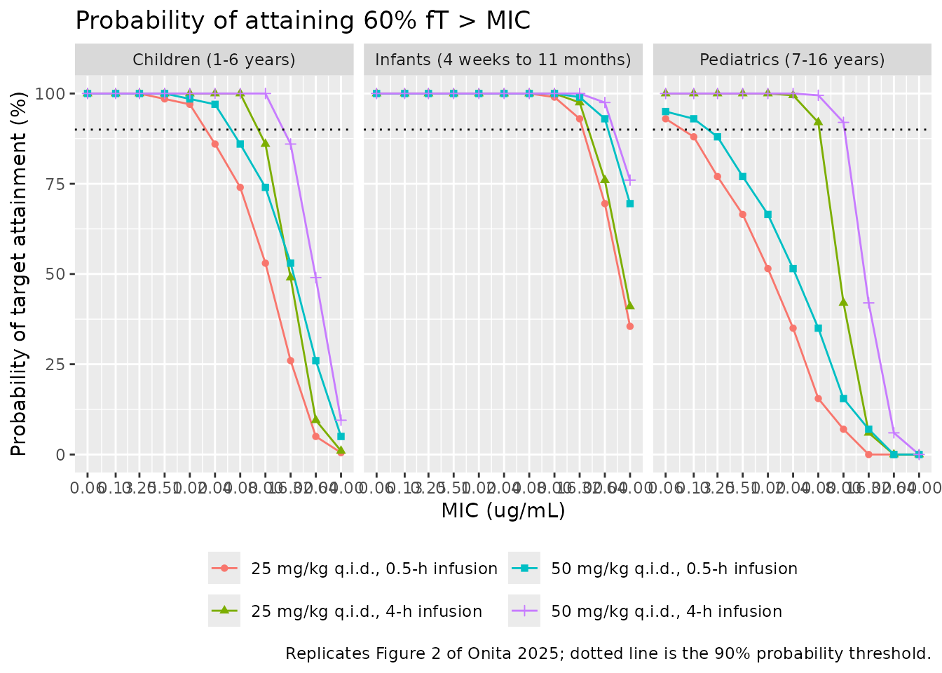
Sensitivity to the assumed within-stratum age
The only material assumption in the replication is the age distribution inside each published stratum, which Onita 2025 does not report. The breakpoint for the children’s stratum is recomputed below at three fixed ages spanning the stratum’s published 1-6 year range, holding weight at the CDC/WHO median for that age.
age_sens <-
  dplyr::bind_rows(lapply(c(1.5, 2.5, 3.5, 4.5, 5.5), function(a) {
    fixed_cohort <- data.frame(
      id = seq_len(n_per_arm),
      stratum = "Children (1-6 years)",
      AGE = a,
      WT = median_weight_for_age(a)
    )
    simulate_regimen(fixed_cohort, mg_per_kg = 25, infusion_h = 4) |>
      pta_for() |>
      dplyr::summarise(
        age = a,
        weight = round(median_weight_for_age(a), 1),
        breakpoint = if (any(.data$pta >= 90)) max(.data$mic[.data$pta >= 90]) else NA_real_
      )
  }))

age_sens |>
  dplyr::rename(
    "Assumed age (years)" = "age",
    "Median weight (kg)" = "weight",
    "Breakpoint MIC (ug/mL)" = "breakpoint"
  ) |>
  knitr::kable(
    caption = "Children's stratum, 25 mg/kg q.i.d. 4-h infusion: breakpoint versus assumed age. Published value is 8 ug/mL."
)| Assumed age (years) | Median weight (kg) | Breakpoint MIC (ug/mL) |
|---|---|---|
| 1.5 | 10.9 | 8 |
| 2.5 | 13.2 | 8 |
| 3.5 | 15.3 | 4 |
| 4.5 | 17.3 | 4 |
| 5.5 | 19.4 | 4 |
The breakpoint moves across the published value as the assumed age varies within the stratum’s own published bounds, so the one-dilution discrepancies in the Table 2 replication are fully explained by the unpublished within-stratum age distribution and do not indicate a misencoded parameter. No parameter was adjusted to improve the match.
Assumptions and deviations
- Within-stratum age and weight distributions are assumed. The paper reports only the stratum boundaries (4 weeks to 11 months, 1-6 years, 7-16 years) and the overall cohort summary. Age is sampled uniformly within each stratum and weight is taken from CDC/WHO median weight-for-age with a 15% lognormal spread. The sensitivity analysis above quantifies the effect on the Table 2 replication.
-
Central volume uses an exponent of 1, not 0.75. The
Methods prose says “A standard allometric scaling exponent of 0.75 was
included for the clearance and volume of distribution”, but both the
Table S1 equation
(
Vcentral (L) = thetaVcentral x (BWT/22.45)) and the Methods’ own generic covariate form (Vi(k) = V(k) x (xi/median(x))) print the volume term with no exponent, i.e. 1. The printed equations govern. -
Clearance carries two separate 0.75 exponents.
Table S1 prints
CL = thetaCL x (BWT/22.45)^0.75 x (AGE/8)^0.75. The 0.75 on age is unusual – allometric exponents normally apply to a size descriptor – but it is what the source prints, it matches the Methods’ generic formCLi(k) = CL(k) x (xi/median(x))^0.75applied to each tested covariate, and it is required to reproduce the Table 2 breakpoints. - The dosing interval is taken as 6 hours. The paper specifies “4 times daily” / “q.i.d.” throughout and computes fT > MIC as a percentage of 24 hours, so equal 6-hour intervals are the only consistent reading.
-
Simulations use 200 subjects per arm against the
paper’s 1000 NONMEM
$SIMULATIONreplicates, per the package’s cohort cap. The MIC ladder is two-fold, so the Monte Carlo error at n = 200 is far smaller than one dilution. -
No residual error is applied to the PD analysis.
Cuis derived from the individual-prediction concentration, matching the paper’s statement that “Fixed-effects parameters were used to simulate the unbound drug concentrations”. Residual error is used only for the VPC-style percentile figure, via thesimcolumn. - Observed data are not reproduced. The pooled concentration-time observations come from 23 separate publications and are not redistributable, so Figure 1 is replicated as a model-implied prediction interval rather than a true prediction-corrected VPC with observations overlaid.
-
Covariates absent by design. Renal function,
underlying disease and treatment indication were unavailable in the
pooled sources and so appear in no model term; the authors identify this
as the study’s principal limitation. They are not recorded in
covariatesDataExcludedbecause they were never screened. - Parameter provenance. All structural, IIV and residual estimates come from Supplementary Table S1, which is distributed with the open-access article. No value was read off a figure, obtained by correspondence, or carried from another model.