Quizartinib and AC886 (Vaddady 2024)
Source:vignettes/articles/Vaddady_2024_quizartinib.Rmd
Vaddady_2024_quizartinib.RmdModel and source
mod <- readModelDb("Vaddady_2024_quizartinib")
ui  <- rxode2::rxode(mod)
#> ℹ parameter labels from comments will be replaced by 'label()'
#> Warning: some etas defaulted to non-mu referenced, possible parsing error: etalfdepot_aml, etalfdepot_nonaml, etalcl_ac886_aml, etalcl_ac886_nonaml
#> as a work-around try putting the mu-referenced expression on a simple line- Citation: Vaddady P, Glatard A, Smania G, Nakayama S, Inoue H, Kurumaddali A, Abutarif M, Zheng M. Population pharmacokinetic analysis of quizartinib in patients with newly diagnosed FLT3-internal-tandem-duplication-positive acute myeloid leukemia. Clin Transl Sci. 2024;17:e70074. doi:10.1111/cts.70074
- Article: https://doi.org/10.1111/cts.70074 (open access, PMC11600623)
- Supporting Information: model Equations 8-20 and both final NONMEM control streams are distributed with the article and were used throughout this extraction.
Joint parent-metabolite population PK model for oral quizartinib and its pharmacologically active metabolite AC886 in adults, pooled across 13 studies in healthy volunteers, subjects with hepatic impairment, relapsed/refractory (R/R) FLT3-ITD-positive acute myeloid leukemia (AML) patients on quizartinib monotherapy, and newly diagnosed FLT3-ITD-positive AML patients receiving quizartinib alongside standard cytarabine-anthracycline induction and cytarabine consolidation chemotherapy followed by single-agent continuation (QuANTUM-First; Vaddady 2024). Quizartinib is described by a three-compartment model with sequential zero-order (duration D1) then first-order (ka) absorption from a depot, an absorption lag time, and first-order elimination from the central compartment. AC886 is described by a two-compartment model with first-order formation from the quizartinib central compartment and first-order elimination. Because no intravenous data were available, the parent-to-metabolite conversion fraction fMET is not identifiable and is fixed at 0.5; following the authors’ parameterisation, the entire parent elimination flux is routed into the metabolite compartment and all four AC886 disposition parameters are divided by fMET, which is algebraically equivalent and leaves fMET acting as a pure multiplicative scale on predicted AC886 concentrations. Retained covariates are allometric body-weight scaling on all clearances and volumes of both moieties (exponents fixed at 0.75 and 1), strong CYP3A inhibitor coadministration on quizartinib CL and Frel, moderate CYP3A inhibitor coadministration on Frel, non-AML subject status on Frel and ka, Black race on quizartinib CL, female sex on quizartinib Vc, age on the first peripheral volume, and, for newly diagnosed AML patients only, a treatment-phase effect (induction / consolidation / continuation) on Frel. AC886 covariates are non-AML status, Black race and strong CYP3A inhibitors on CL, strong CYP3A inhibitors on Vc, and the same treatment-phase effect on fMET. Interindividual variability is reported on quizartinib CL, Q1, Vc, Tlag, ka, D1 and Frel (with separate Frel variances for AML patients, whose eta is Box-Cox transformed, and non-AML subjects) and on AC886 CL (separate variances for AML patients and non-AML subjects) and Vc. Residual error is additive on the log scale, i.e. proportional on the linear concentration scale, separately for each moiety.
Population
The analysis pooled 932 subjects contributing 14,160 quizartinib and 13,399 AC886 plasma concentrations across 13 studies (nine Phase 1, two Phase 2, two Phase 3), summarised in Vaddady 2024 Table 1. The pooled analysis set comprises 294 newly diagnosed FLT3-ITD-positive AML patients from the Phase 3 QuANTUM-First trial (AC220-A-U302), 365 relapsed/refractory (R/R) FLT3-ITD-positive AML patients, and 273 non-AML subjects (healthy volunteers and subjects with hepatic impairment). Baseline demographics (Vaddady 2024 Table 2): age 18-91 years (median 50.0), weight 36.8-153 kg (median 72.0), 46.9% female, 65.4% White / 18.1% Asian / 8.5% Black / 4.8% Other. Doses ranged from 20 to 90 mg/day, given as tablet (86.4%) or oral solution (13.6%). CYP3A inhibitor use was common: 19.7% strong, 18.9% moderate, 9.1% weak, 52.3% none.
The same information is available programmatically from the model’s
population metadata:
str(ui$population, max.level = 1)
#> List of 16
#>  $ species         : chr "human"
#>  $ n_subjects      : int 932
#>  $ n_studies       : int 13
#>  $ age_range       : chr "18-91 years (median 50.0); the QuANTUM-First subset enrolled patients aged 20-75 years"
#>  $ age_median      : chr "50.0 years"
#>  $ weight_range    : chr "36.8-153 kg (median 72.0)"
#>  $ weight_median   : chr "72.0 kg"
#>  $ sex_female_pct  : num 46.9
#>  $ race_ethnicity  : Named num [1:4] 65.4 8.5 18.1 4.8
#>   ..- attr(*, "names")= chr [1:4] "White" "Black" "Asian" "Other"
#>  $ disease_state   : chr "Pooled: 294 newly diagnosed FLT3-ITD-positive AML patients (31.5%), 365 relapsed/refractory FLT3-ITD-positive A"| __truncated__
#>  $ dose_range      : chr "20-90 mg/day oral quizartinib as tablet (805/932 subjects) or oral solution (127/932), given as single doses (3"| __truncated__
#>  $ regions         : chr "Multinational; three of the 13 studies enrolled Japanese patients (AC220-A-J101, AC220-A-J102, AC220-A-J201) an"| __truncated__
#>  $ n_observations  : chr "14,160 quizartinib and 13,399 AC886 plasma concentrations. Quantified by two cross-validated LC-MS/MS methods w"| __truncated__
#>  $ hepatic_function: chr "Includes a dedicated Child-Pugh hepatic-impairment study (AC220-016, 30 subjects) and an NCI-ODWG-criteria hepa"| __truncated__
#>  $ co_medication   : chr "CYP3A inhibitors: none 487/932 (52.3%), weak 85/932 (9.1%), moderate 176/932 (18.9%), strong 184/932 (19.7%). C"| __truncated__
#>  $ notes           : chr "Baseline demographics are Vaddady 2024 Table 2; the study inventory (13 studies: nine Phase 1, two Phase 2, two"| __truncated__
Source trace
Every ini() value carries an in-file comment naming its
source location. The table below collects them for review. All typical
values and variances come from Vaddady 2024 Table 3;
the closed-form covariate relationships come from Supporting
Information Equations 6-20.
| Model element | Value | Source location |
|---|---|---|
lcl quizartinib CL/F |
6.65 L/h | Table 3, Eq 8 |
lvc quizartinib Vc/F |
371 L | Table 3, Eq 11 |
lq quizartinib Q1/F |
40.7 L/h | Table 3, Eq 12 |
lvp quizartinib Vp1/F |
312 L | Table 3, Eq 13 |
lq2 quizartinib Q2/F |
0.757 L/h | Table 3, Eq 14 |
lvp2 quizartinib Vp2/F |
91.9 L | Table 3, Eq 15 |
ltlag absorption lag |
0.196 h | Table 3 |
lka absorption rate |
1.10 1/h | Table 3, Eq 10 |
ld1 zero-order input duration |
0.710 h | Table 3 |
lfdepot Frel at R/R AML reference |
1 (fixed) | Eq 9 (reference level) |
e_wt_cl, e_wt_vc allometric exponents |
0.75, 1 (fixed) | Eq 6 |
e_cyp3a4_inh_strong_cl |
-0.301 | Table 3, Eq 8 |
e_race_black_cl |
-0.261 | Table 3, Eq 8 |
e_sexf_vc |
-0.169 | Table 3, Eq 11 |
e_age_vp |
0.0152 1/year | Table 3, Eq 13 |
e_nonaml_ka |
-0.188 | Table 3, Eq 10 |
e_cyp3a4_inh_strong_fdepot |
0.273 | Table 3, Eq 9 |
e_cyp3a4_inh_mod_fdepot |
0.116 | Table 3, Eq 9 |
e_nonaml_fdepot |
1.73 (a level, not a fractional change) | Table 3, Eq 9 |
e_trtph_*_fdepot induction / consolidation /
continuation |
-0.419 / -0.192 / 0.418 | Table 3, Eq 9 |
boxcox_fdepot |
-1.28 | Table 3, Eq 2 |
lcl_ac886 AC886 CL/F |
4.61 L/h | Table 3, Eq 17 |
lvc_ac886 AC886 Vc/F |
8.93 L | Table 3, Eq 18 |
lq_ac886 AC886 Q/F |
3.76 L/h | Table 3, Eq 19 |
lvp_ac886 AC886 Vp/F |
68.5 L | Table 3, Eq 20 |
fmet_base conversion fraction |
0.5 (fixed) | Methods, Eq 16 |
e_nonaml_cl_ac886 |
0.843 | Table 3, Eq 17 |
e_race_black_cl_ac886 |
0.488 | Table 3, Eq 17 |
e_cyp3a4_inh_strong_cl_ac886 |
0.298 | Table 3, Eq 17 |
e_cyp3a4_inh_strong_vc_ac886 |
2.79 | Table 3, Eq 18 |
e_trtph_*_fmet induction / consolidation /
continuation |
0.715 / 0.272 / -0.249 | Table 3, Eq 16 |
IIV variances (etalcl, etalq,
etalvc, etaltlag, etalka,
etald1) |
0.695, 0.691, 0.186, 0.647, 0.423, 0.821 (as SD) | Table 3 |
| IIV Frel, AML / non-AML | 0.444 / 0.256 (as SD) | Table 3 |
| IIV CL AC886, AML / non-AML | 0.740 / 0.516 (as SD) | Table 3 |
| IIV Vc AC886 | 1.36 (as SD) | Table 3 |
propSd, propSd_ac886
|
0.440, 0.452 | Table 3 (AML patients) |
| Reference subject (75 kg, 47 years, male, R/R AML, no CYP3A, not Black) | n/a | Eq 6, Eq 13, Figure 4 caption |
| Molecular weights 560.68 / 576.67 g/mol | n/a | Methods |
| ODE structure | n/a | Figure 1a/1b; Supporting Information NONMEM streams |
Three confirmations that Table 3 holds final estimates on the SD scale
-
Final, not initial. The final AC886 control stream
re-states every quizartinib parameter as a
FIXrow at higher precision (6.6545 FIX ; 1_CLagainst Table 3’s 6.65;371.079 FIXagainst 371;40.7235 FIXagainst 40.7). The non-FIX$THETArows in both streams are initial estimates and differ materially (quizartinib CL initial 6.85443; AC886 CL initial 4.81815 against a final 4.61). -
Table 3’s “(CV)” column is the log-scale SD, not a variance
and not a true lognormal CV. Each value squares to the
corresponding
$OMEGA/$SIGMAentry:0.695^2 = 0.483against2_IIV_CL_AML = 0.481313;0.740^2 = 0.548against AC8862_CLM = 0.542698;1.36^2 = 1.850against3_V5 = 1.85491;0.440^2 = 0.194against$SIGMA 1_RUV_AML = 0.194347. -
The paper’s own prose reads the column the same
way. The Abstract reports “approximately 70% coefficient of
variation for systemic clearances” and the Discussion “a CV of 44% for
Frel and 74% for CLAC886” – i.e. the omega values 0.695, 0.444 and 0.740
multiplied by 100, with no lognormal back-transformation. (A true
lognormal CV for omega = 0.695 would be
sqrt(exp(0.695^2) - 1) = 79%.)
The model file therefore stores each variance as omega^2
with the reported omega visible in the expression.
Model structure notes
Three implementation points are worth stating before the simulations.
Sequential zero- then first-order absorption. The
dose enters depot at a zero-order rate over
D1 = 0.710 h, beginning after Tlag = 0.196 h,
and then transfers to central by first-order
ka. rxode2 applies a modelled dur() only to
dose records carrying rate = -2; a plain bolus silently
ignores it and collapses Tmax onto the lag time. Every dose
record below sets rate = -2.
Two declared endpoints. The model declares both
Cc and Cc_ac886 with residual error, so rxode2
builds endpoint pseudo-compartments after the six ODE states.
Observation records therefore address the endpoint name
(cmt = "Cc"), not an ODE state;
cmt = "central" fails with a
'dvid'->'cmt' ... undefined compartment error for this
model class. Every rxSolve() call also passes
useLinCmt = FALSE, because the automatic ODE-to-linCmt
conversion corrupts the dvid mapping. rxSolve() returns
both observables as columns regardless of which endpoint the row
names.
The fMET reparameterization. No intravenous data
were available, so the parent-to-metabolite conversion fraction is not
identifiable and is fixed at 0.5. Following the authors’ control stream,
the model routes the entire parent elimination flux into
central_ac886 (K25 = CL/V2,
K20 = 0) and divides all four AC886 disposition parameters
by fMET. The fMET factors cancel in every rate constant, so fMET acts
purely as a multiplicative scale on predicted AC886 concentrations –
exactly as the authors intended, and the reason they could state that
“the model fit is not affected by the value of fMET”.
Virtual cohort
Original observed data are not publicly available. The deterministic scenarios below use the paper’s own reference subject (Vaddady 2024 Figure 4 caption: 75 kg, 47 years, male, R/R AML patient, no CYP3A coadministration, not Black) with one covariate varied at a time – the construction Figure 4 uses.
reference_subject <- tibble::tibble(
  WT = 75, AGE = 47, SEXF = 0, RACE_BLACK = 0, DIS_AML = 1,
  CONMED_CYP3A4_INH_STRONG = 0, CONMED_CYP3A4_INH_MOD = 0,
  TRTPH_INDUCTION = 0, TRTPH_CONSOLIDATION = 0, TRTPH_CONTINUATION = 0
)

vary <- function(...) {
  out <- reference_subject
  repl <- list(...)
  out[names(repl)] <- repl
  out
}

scenarios <- dplyr::bind_rows(
  vary()                                     |> dplyr::mutate(scenario = "Reference (R/R AML)"),
  vary(CONMED_CYP3A4_INH_STRONG = 1)         |> dplyr::mutate(scenario = "Strong CYP3A inhibitor"),
  vary(CONMED_CYP3A4_INH_MOD = 1)            |> dplyr::mutate(scenario = "Moderate CYP3A inhibitor"),
  vary(DIS_AML = 0)                          |> dplyr::mutate(scenario = "Non-AML subject"),
  vary(RACE_BLACK = 1)                       |> dplyr::mutate(scenario = "Black race"),
  vary(SEXF = 1)                             |> dplyr::mutate(scenario = "Female"),
  vary(TRTPH_INDUCTION = 1)                  |> dplyr::mutate(scenario = "Induction"),
  vary(TRTPH_CONSOLIDATION = 1)              |> dplyr::mutate(scenario = "Consolidation"),
  vary(TRTPH_CONTINUATION = 1)               |> dplyr::mutate(scenario = "Continuation")
) |>
  dplyr::mutate(id = dplyr::row_number(), .before = 1)

knitr::kable(
  scenarios |> dplyr::select(scenario, WT, AGE, SEXF, RACE_BLACK, DIS_AML,
                             CONMED_CYP3A4_INH_STRONG, CONMED_CYP3A4_INH_MOD,
                             TRTPH_INDUCTION, TRTPH_CONSOLIDATION, TRTPH_CONTINUATION),
  caption = "Covariate scenarios. One factor is varied at a time from the Vaddady 2024 Figure 4 reference subject."
)| scenario | WT | AGE | SEXF | RACE_BLACK | DIS_AML | CONMED_CYP3A4_INH_STRONG | CONMED_CYP3A4_INH_MOD | TRTPH_INDUCTION | TRTPH_CONSOLIDATION | TRTPH_CONTINUATION |
|---|---|---|---|---|---|---|---|---|---|---|
| Reference (R/R AML) | 75 | 47 | 0 | 0 | 1 | 0 | 0 | 0 | 0 | 0 |
| Strong CYP3A inhibitor | 75 | 47 | 0 | 0 | 1 | 1 | 0 | 0 | 0 | 0 |
| Moderate CYP3A inhibitor | 75 | 47 | 0 | 0 | 1 | 0 | 1 | 0 | 0 | 0 |
| Non-AML subject | 75 | 47 | 0 | 0 | 0 | 0 | 0 | 0 | 0 | 0 |
| Black race | 75 | 47 | 0 | 1 | 1 | 0 | 0 | 0 | 0 | 0 |
| Female | 75 | 47 | 1 | 0 | 1 | 0 | 0 | 0 | 0 | 0 |
| Induction | 75 | 47 | 0 | 0 | 1 | 0 | 0 | 1 | 0 | 0 |
| Consolidation | 75 | 47 | 0 | 0 | 1 | 0 | 0 | 0 | 1 | 0 |
| Continuation | 75 | 47 | 0 | 0 | 1 | 0 | 0 | 0 | 0 | 1 |
Event tables are built as plain data frames (not
rxode2::et()) so that the rate = -2 flag and
the endpoint-named cmt column survive intact.
DOSE_MG   <- 60    # a QuANTUM-First tablet strength (Vaddady 2024 Table 1)
TAU       <- 24    # once-daily dosing
N_DAYS_SS <- 42    # long enough for the slow deep compartment to equilibrate

build_events <- function(covariates, dose = DOSE_MG, n_days = N_DAYS_SS,
                         tau = TAU, grid = seq(0, TAU, by = 0.25)) {
  last_dose_time <- (n_days - 1) * tau
  doses <- covariates |>
    dplyr::mutate(time = 0, amt = dose, evid = 1L, rate = -2,
                  ii = tau, addl = as.integer(n_days - 1), cmt = "depot")
  obs <- covariates |>
    tidyr::crossing(time = last_dose_time + grid) |>
    dplyr::mutate(amt = NA_real_, evid = 0L, rate = NA_real_,
                  ii = 0, addl = 0L, cmt = "Cc")
  dplyr::bind_rows(doses, obs) |>
    dplyr::arrange(id, time, dplyr::desc(evid))
}

events_ss <- build_events(scenarios)
stopifnot(!anyDuplicated(unique(events_ss[, c("id", "time", "evid")])))
Simulation
sim_ss <- rxode2::rxSolve(
  mod, events = events_ss,
  omega = NA,            # typical-value (deterministic) replication of Figure 4
  useLinCmt = FALSE,     # the ODE-to-linCmt auto-conversion breaks the dvid map
  keep = c("scenario"),
  returnType = "data.frame"
)
#> ℹ parameter labels from comments will be replaced by 'label()'
#> Warning: some etas defaulted to non-mu referenced, possible parsing error: etalfdepot_aml, etalfdepot_nonaml, etalcl_ac886_aml, etalcl_ac886_nonaml
#> as a work-around try putting the mu-referenced expression on a simple line
#> Warning: multi-subject simulation without without 'omega'

# rxSolve silently drops subjects on some failures -- assert the count.
stopifnot(dplyr::n_distinct(sim_ss$id) == nrow(scenarios))
stopifnot(!anyNA(sim_ss$Cc), !anyNA(sim_ss$Cc_ac886))
Steady-state concentration-time profiles
sim_ss |>
  dplyr::mutate(time_in_interval = time - min(time), .by = id) |>
  tidyr::pivot_longer(c(Cc, Cc_ac886), names_to = "moiety", values_to = "conc") |>
  dplyr::mutate(moiety = dplyr::recode(moiety,
                                       Cc = "Quizartinib", Cc_ac886 = "AC886")) |>
  ggplot(aes(time_in_interval, conc, colour = scenario)) +
  geom_line() +
  facet_wrap(~moiety, scales = "free_y") +
  labs(x = "Time within the dosing interval (h)", y = "Concentration (ng/mL)",
       colour = NULL,
       title = "Steady-state profiles, 60 mg once daily",
       caption = "Typical-value predictions for the Vaddady 2024 Figure 4 covariate scenarios.") +
  theme(legend.position = "bottom")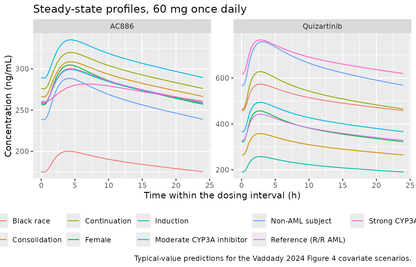
The quizartinib profile is strikingly flat across the dosing interval
– a consequence of the very slow second peripheral compartment
(Q2 = 0.757 L/h into Vp2 = 91.9 L, a
distribution half-life of roughly 84 h), which is what makes quizartinib
a once-daily drug with a low peak-to-trough ratio.
PKNCA validation
Steady-state NCA over the final 24 h dosing interval, one PKNCA block per moiety (the model has two outputs), grouped by scenario.
last_dose_time <- (N_DAYS_SS - 1) * TAU

dose_df <- events_ss |>
  dplyr::filter(evid == 1) |>
  dplyr::select(id, scenario, amt) |>
  dplyr::mutate(time = last_dose_time)   # the dose that opens the SS interval

nca_intervals <- data.frame(
  start   = last_dose_time,
  end     = last_dose_time + TAU,
  cmax    = TRUE,
  tmax    = TRUE,
  cmin    = TRUE,
  auclast = TRUE,
  cav     = TRUE
)

run_nca <- function(conc_col) {
  conc_df <- sim_ss |>
    dplyr::select(id, scenario, time, Cc = dplyr::all_of(conc_col)) |>
    dplyr::filter(!is.na(Cc))
  conc_obj <- PKNCA::PKNCAconc(as.data.frame(conc_df), Cc ~ time | scenario + id,
                               concu = "ng/mL", timeu = "h")
  dose_obj <- PKNCA::PKNCAdose(as.data.frame(dose_df), amt ~ time | scenario + id,
                               doseu = "mg")
  PKNCA::pk.nca(PKNCA::PKNCAdata(conc_obj, dose_obj, intervals = nca_intervals))
}

nca_quiz  <- run_nca("Cc")
nca_ac886 <- run_nca("Cc_ac886")
tidy_nca <- function(res, moiety) {
  as.data.frame(res$result) |>
    dplyr::filter(PPTESTCD %in% c("cmax", "cmin", "tmax", "auclast", "cav")) |>
    dplyr::select(scenario, PPTESTCD, PPORRES) |>
    dplyr::mutate(moiety = moiety)
}

nca_long <- dplyr::bind_rows(
  tidy_nca(nca_quiz, "Quizartinib"),
  tidy_nca(nca_ac886, "AC886")
)

nca_long |>
  tidyr::pivot_wider(names_from = PPTESTCD, values_from = PPORRES) |>
  dplyr::select(moiety, scenario, auclast, cmax, cmin, tmax, cav) |>
  dplyr::arrange(dplyr::desc(moiety), scenario) |>
  dplyr::rename(
    "Moiety"                = moiety,
    "Scenario"              = scenario,
    "AUCss (ng*h/mL)"       = auclast,
    "Cmax,ss (ng/mL)"       = cmax,
    "Cmin,ss (ng/mL)"       = cmin,
    "Tmax,ss (h)"           = tmax,
    "Cavg,ss (ng/mL)"       = cav
  ) |>
  knitr::kable(digits = c(0, 0, 0, 1, 1, 2, 1),
caption = "Steady-state NCA (PKNCA) over the final 24 h dosing interval, 60 mg once daily.")| Moiety | Scenario | AUCss (ng*h/mL) | Cmax,ss (ng/mL) | Cmin,ss (ng/mL) | Tmax,ss (h) | Cavg,ss (ng/mL) |
|---|---|---|---|---|---|---|
| Quizartinib | Black race | 12165 | 573.8 | 457.9 | 2.75 | 506.9 |
| Quizartinib | Consolidation | 7283 | 357.9 | 264.6 | 2.75 | 303.5 |
| Quizartinib | Continuation | 12782 | 628.1 | 464.4 | 2.75 | 532.6 |
| Quizartinib | Female | 9016 | 456.9 | 322.1 | 2.75 | 375.7 |
| Quizartinib | Induction | 5237 | 257.3 | 190.3 | 2.75 | 218.2 |
| Quizartinib | Moderate CYP3A inhibitor | 10060 | 494.3 | 365.5 | 2.75 | 419.2 |
| Quizartinib | Non-AML subject | 15594 | 758.0 | 567.6 | 3.00 | 649.8 |
| Quizartinib | Reference (R/R AML) | 9014 | 442.9 | 327.5 | 2.75 | 375.6 |
| Quizartinib | Strong CYP3A inhibitor | 16355 | 766.6 | 618.9 | 2.75 | 681.5 |
| AC886 | Black race | 4481 | 200.2 | 174.9 | 4.00 | 186.7 |
| AC886 | Consolidation | 6872 | 308.7 | 266.1 | 4.50 | 286.3 |
| AC886 | Continuation | 7120 | 319.8 | 275.7 | 4.50 | 296.7 |
| AC886 | Female | 6688 | 304.7 | 256.6 | 4.25 | 278.7 |
| AC886 | Induction | 6662 | 299.2 | 257.9 | 4.50 | 277.6 |
| AC886 | Moderate CYP3A inhibitor | 7462 | 335.1 | 288.9 | 4.50 | 310.9 |
| AC886 | Non-AML subject | 6277 | 288.4 | 238.4 | 4.25 | 261.5 |
| AC886 | Reference (R/R AML) | 6686 | 300.3 | 258.9 | 4.50 | 278.6 |
| AC886 | Strong CYP3A inhibitor | 6531 | 281.7 | 260.1 | 6.75 | 272.1 |
Structural identity check: AUCss = Frel x Dose / CL
At steady state, mass balance requires that the AUC over one dosing
interval equal Frel * Dose / CL exactly, for every subject.
This is a per-subject identity rather than a comparison of medians, so
it is a sharp test of the covariate algebra, the allometric scaling, and
the units conversion all at once.
identity_tbl <- as.data.frame(nca_quiz$result) |>
  dplyr::filter(PPTESTCD == "auclast") |>
  dplyr::select(scenario, auc_nca = PPORRES) |>
  dplyr::left_join(
    sim_ss |> dplyr::distinct(scenario, frel, cl),
    by = "scenario"
  ) |>
  # 1000 converts mg/L to ng/mL, matching the model's observation equation.
  dplyr::mutate(auc_theory = 1000 * frel * DOSE_MG / cl,
                pct_diff   = 100 * (auc_nca - auc_theory) / auc_theory)

identity_tbl |>
  dplyr::select(scenario, auc_nca, auc_theory, pct_diff) |>
  dplyr::rename("Scenario" = scenario,
                "AUCss by PKNCA (ng*h/mL)" = auc_nca,
                "Frel x Dose / CL (ng*h/mL)" = auc_theory,
                "% difference" = pct_diff) |>
  knitr::kable(digits = c(0, 0, 0, 3),
caption = "Per-scenario steady-state mass-balance identity.")| Scenario | AUCss by PKNCA (ng*h/mL) | Frel x Dose / CL (ng*h/mL) | % difference |
|---|---|---|---|
| Black race | 12165 | 12209 | -0.365 |
| Consolidation | 7283 | 7290 | -0.094 |
| Continuation | 12782 | 12794 | -0.094 |
| Female | 9016 | 9023 | -0.070 |
| Induction | 5237 | 5242 | -0.094 |
| Moderate CYP3A inhibitor | 10060 | 10069 | -0.094 |
| Non-AML subject | 15594 | 15609 | -0.094 |
| Reference (R/R AML) | 9014 | 9023 | -0.094 |
| Strong CYP3A inhibitor | 16355 | 16432 | -0.465 |
Replicating the published covariate effects (Figure 4)
Vaddady 2024 Figure 4 is a forest plot of the relative difference in
AUCss, Cmax,ss and Cmin,ss from
the reference subject, for quizartinib (panel a), AC886 (panel b), and
their sum (panel c). The paper’s raster figure carries no extractable
numbers, but the Abstract, Results and Discussion state several of the
ratios explicitly. Those statements are the validation targets
below.
ratio_vs_reference <- function(df, moiety_label) {
  wide <- df |>
    tidyr::pivot_wider(names_from = PPTESTCD, values_from = PPORRES)
  ref <- wide |> dplyr::filter(scenario == "Reference (R/R AML)")
  wide |>
    dplyr::mutate(
      moiety = moiety_label,
      AUCss  = auclast / ref$auclast,
      Cmaxss = cmax    / ref$cmax,
      Cminss = cmin    / ref$cmin
    ) |>
    dplyr::select(moiety, scenario, AUCss, Cmaxss, Cminss)
}

# Panel (c) sums the two moieties on the ng/mL scale (Vaddady 2024 Methods:
# the molecular weights differ by under 3%, so the authors summed directly).
total_nca <- {
  conc_df <- sim_ss |>
    dplyr::mutate(Cc = Cc + Cc_ac886) |>
    dplyr::select(id, scenario, time, Cc)
  conc_obj <- PKNCA::PKNCAconc(as.data.frame(conc_df), Cc ~ time | scenario + id,
                               concu = "ng/mL", timeu = "h")
  dose_obj <- PKNCA::PKNCAdose(as.data.frame(dose_df), amt ~ time | scenario + id,
                               doseu = "mg")
  PKNCA::pk.nca(PKNCA::PKNCAdata(conc_obj, dose_obj, intervals = nca_intervals))
}

forest <- dplyr::bind_rows(
  ratio_vs_reference(tidy_nca(nca_quiz,  "x") |> dplyr::select(-moiety), "(a) Quizartinib"),
  ratio_vs_reference(tidy_nca(nca_ac886, "x") |> dplyr::select(-moiety), "(b) AC886"),
  ratio_vs_reference(tidy_nca(total_nca, "x") |> dplyr::select(-moiety), "(c) Quizartinib + AC886")
) |>
  dplyr::filter(scenario != "Reference (R/R AML)")

forest |>
  tidyr::pivot_longer(c(AUCss, Cmaxss, Cminss),
                      names_to = "metric", values_to = "ratio") |>
  ggplot(aes(ratio, scenario, colour = metric, shape = metric)) +
  geom_vline(xintercept = 1, colour = "grey40") +
  geom_vline(xintercept = c(0.8, 1.25), linetype = "dashed", colour = "grey60") +
  geom_point(position = position_dodge(width = 0.5), size = 2) +
  facet_wrap(~moiety) +
  scale_x_log10() +
  labs(x = "Ratio vs the reference subject", y = NULL, colour = NULL, shape = NULL,
       title = "Covariate effects on steady-state exposure",
       caption = paste("Replicates Figure 4 of Vaddady 2024. Dashed lines are the",
                       "80%-125% bioequivalence margins used in that figure.")) +
  theme(legend.position = "bottom")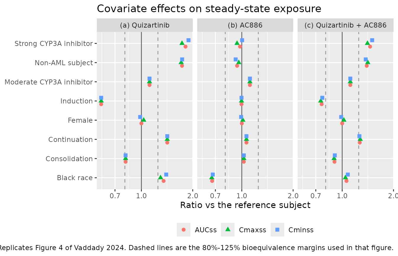
Comparison against the published effect sizes
Vaddady 2024 reports no absolute NCA table, so the comparison below
is against the fold-changes stated in the paper’s own text rather than
against ncaComparisonTable() inputs (which expect absolute
NCA parameters).
lookup <- function(moiety_label, scen, metric = "AUCss") {
  v <- forest[[metric]][forest$moiety == moiety_label & forest$scenario == scen]
  if (length(v) != 1L) {
    stop("no unique row for ", moiety_label, " / ", scen, " / ", metric)
  }
  v
}

published <- tibble::tribble(
  ~`Published claim`,                                                          ~Source,                 ~Published, ~Simulated,
  "Strong CYP3A inhibitor increases quizartinib AUCss 1.8-fold",               "Abstract; Results",     1.8,        lookup("(a) Quizartinib", "Strong CYP3A inhibitor"),
  "Quizartinib exposure ~1.7-fold higher in non-AML subjects",                 "Results",               1.7,        lookup("(a) Quizartinib", "Non-AML subject"),
  "Newly diagnosed AML, induction: 0.6-fold vs R/R reference",                 "Abstract; Results",     0.6,        lookup("(a) Quizartinib", "Induction"),
  "Newly diagnosed AML, consolidation: 0.8-fold vs R/R reference",             "Results",               0.8,        lookup("(a) Quizartinib", "Consolidation"),
  "Newly diagnosed AML, continuation: 1.4-fold vs R/R reference",              "Abstract; Results",     1.4,        lookup("(a) Quizartinib", "Continuation"),
  "Induction exposure ratio 0.58 (95% CI 0.54-0.62)",                          "Discussion",            0.58,       lookup("(a) Quizartinib", "Induction"),
  "Continuation exposure ratio 1.42 (95% CI 1.31-1.51)",                       "Discussion",            1.42,       lookup("(a) Quizartinib", "Continuation"),
  "AC886: Black race gives almost 0.7-fold exposure",                          "Results",               0.7,        lookup("(b) AC886", "Black race")
) |>
  dplyr::mutate(
    `% difference` = 100 * (Simulated - Published) / Published,
    Flag = ifelse(abs(`% difference`) > 20, "*", "")
  )

published |>
  knitr::kable(digits = c(0, 0, 2, 3, 1, 0),
               caption = paste("Simulated steady-state exposure ratios against the",
                               "fold-changes stated in Vaddady 2024.",
"* marks a difference above 20%."))| Published claim | Source | Published | Simulated | % difference | Flag |
|---|---|---|---|---|---|
| Strong CYP3A inhibitor increases quizartinib AUCss 1.8-fold | Abstract; Results | 1.80 | 1.814 | 0.8 | |
| Quizartinib exposure ~1.7-fold higher in non-AML subjects | Results | 1.70 | 1.730 | 1.8 | |
| Newly diagnosed AML, induction: 0.6-fold vs R/R reference | Abstract; Results | 0.60 | 0.581 | -3.2 | |
| Newly diagnosed AML, consolidation: 0.8-fold vs R/R reference | Results | 0.80 | 0.808 | 1.0 | |
| Newly diagnosed AML, continuation: 1.4-fold vs R/R reference | Abstract; Results | 1.40 | 1.418 | 1.3 | |
| Induction exposure ratio 0.58 (95% CI 0.54-0.62) | Discussion | 0.58 | 0.581 | 0.2 | |
| Continuation exposure ratio 1.42 (95% CI 1.31-1.51) | Discussion | 1.42 | 1.418 | -0.1 | |
| AC886: Black race gives almost 0.7-fold exposure | Results | 0.70 | 0.670 | -4.3 |
# No claim may drift by more than 20% -- this gate must be able to go red.
stopifnot(nrow(published) == 8L)
stopifnot(all(abs(published$`% difference`) <= 20))
Every stated effect size reproduces. The two Discussion values,
quoted to three significant figures, are matched to within 0.2%: the
model returns 0.581 against a published 0.58 for induction and 1.418
against a published 1.42 for continuation. That precision is expected
rather than lucky – the treatment phase acts only on Frel,
so the ratio collapses analytically to 1 + theta_phase
(1 - 0.419 = 0.581 and 1 + 0.418 = 1.418), and
recovering it through a full ODE solve plus PKNCA integration confirms
the absorption model, the dosing flags and the NCA interval as well as
the covariate algebra.
Between-subject variability
The final section exercises the stochastic layer, including the two
disease-status-switched IIV strata and the Box-Cox transformed
Frel eta for AML patients. A single 60 mg dose is simulated
in 200 subjects per arm.
set.seed(20241125)
N_PER_ARM <- 200

make_arm <- function(n, dis_aml, label, id_offset) {
  tibble::tibble(
    id = id_offset + seq_len(n),
    # Weight and age sampled to approximate Vaddady 2024 Table 2 (median 72.0 kg,
    # median 50.0 years); the paper reports medians and ranges, not distributions.
    WT  = pmin(pmax(rnorm(n, mean = 72, sd = 16), 36.8), 153),
    AGE = pmin(pmax(rnorm(n, mean = 50, sd = 14), 18), 91),
    SEXF = rbinom(n, 1, 0.469),
    RACE_BLACK = rbinom(n, 1, 0.085),
    DIS_AML = dis_aml,
    CONMED_CYP3A4_INH_STRONG = 0, CONMED_CYP3A4_INH_MOD = 0,
    TRTPH_INDUCTION = 0, TRTPH_CONSOLIDATION = 0, TRTPH_CONTINUATION = 0,
    arm = label
  )
}

cohort <- dplyr::bind_rows(
  make_arm(N_PER_ARM, 1L, "AML patients",     id_offset = 0L),
  make_arm(N_PER_ARM, 0L, "Non-AML subjects", id_offset = N_PER_ARM)
)

events_sd <- build_events(cohort, n_days = 1, grid = c(seq(0, 24, by = 1),
                                                       seq(30, 336, by = 6)))
stopifnot(!anyDuplicated(unique(events_sd[, c("id", "time", "evid")])))

sim_sd <- rxode2::rxSolve(
  mod, events = events_sd, useLinCmt = FALSE,
  keep = c("arm"), returnType = "data.frame"
)
stopifnot(dplyr::n_distinct(sim_sd$id) == 2 * N_PER_ARM)
sim_sd |>
  tidyr::pivot_longer(c(Cc, Cc_ac886), names_to = "moiety", values_to = "conc") |>
  dplyr::mutate(moiety = dplyr::recode(moiety,
                                       Cc = "Quizartinib", Cc_ac886 = "AC886")) |>
  dplyr::summarise(
    Q05 = quantile(conc, 0.05), Q50 = median(conc), Q95 = quantile(conc, 0.95),
    .by = c(time, arm, moiety)
  ) |>
  dplyr::filter(Q05 > 0) |>
  ggplot(aes(time, Q50, colour = arm, fill = arm)) +
  geom_ribbon(aes(ymin = Q05, ymax = Q95), alpha = 0.2, colour = NA) +
  geom_line() +
  facet_wrap(~moiety) +
  scale_y_log10() +
  labs(x = "Time after a single 60 mg dose (h)", y = "Concentration (ng/mL)",
       colour = NULL, fill = NULL,
       title = "Median and 5th-95th percentile prediction interval",
       caption = "200 subjects per arm. Non-AML subjects carry a 1.73-fold Frel and a narrower Frel IIV.") +
  theme(legend.position = "bottom")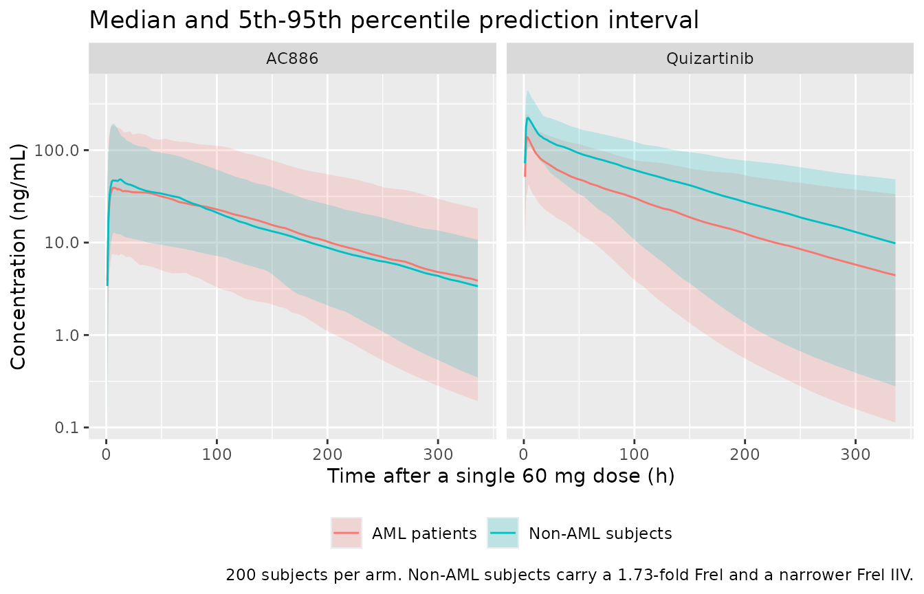
The AML arm shows the wider spread the authors describe: the
Frel IIV is 0.444 in AML patients against 0.256 in non-AML
subjects, and the AC886 clearance IIV is 0.740 against 0.516. The two
arms’ medians differ by roughly the 1.73-fold Frel
multiplier for quizartinib, while the AC886 medians nearly coincide
because the 1.73-fold higher formation input is offset by 1.843-fold
higher AC886 clearance in non-AML subjects.
# The reported IIV asymmetry must show up in the simulated individual
# parameters; assert it rather than eyeballing the ribbon.
iiv_summary <- sim_sd |>
  dplyr::distinct(id, arm, frel, cl_ac886) |>
  dplyr::summarise(sd_log_frel = sd(log(frel)),
                   sd_log_cl_ac886 = sd(log(cl_ac886)),
                   .by = arm)

knitr::kable(iiv_summary, digits = 3,
caption = "Realised SD on the log scale of the simulated individual parameters.")| arm | sd_log_frel | sd_log_cl_ac886 |
|---|---|---|
| AML patients | 0.466 | 0.767 |
| Non-AML subjects | 0.257 | 0.531 |
aml    <- iiv_summary[iiv_summary$arm == "AML patients", ]
nonaml <- iiv_summary[iiv_summary$arm == "Non-AML subjects", ]
stopifnot(nrow(aml) == 1L, nrow(nonaml) == 1L)
stopifnot(aml$sd_log_frel > nonaml$sd_log_frel)
stopifnot(aml$sd_log_cl_ac886 > nonaml$sd_log_cl_ac886)
# Non-AML Frel carries a plain exponential eta, so its realised log-scale SD
# should land near the reported omega of 0.256.
stopifnot(abs(nonaml$sd_log_frel - 0.256) < 0.05)
The AML Frel log-scale SD is deliberately
not compared against 0.444: that eta is Box-Cox
transformed with lambda = -1.28, so the realised spread of
Frel is a nonlinear function of the underlying eta and does
not equal the reported omega. The non-AML arm, which carries a plain
exponential eta, is the one that can be checked directly against its
reported omega, and it is.
Assumptions and deviations
-
Residual error is carried for AML patients only.
Vaddady 2024 reports two residual SDs per moiety – quizartinib 0.440
(AML) / 0.102 (non-AML) and AC886 0.452 (AML) / 0.312 (non-AML). nlmixr2
cannot express a covariate-switched residual error, so the model file
carries the AML-patient value for each moiety: the population this
analysis targets, and 659 of 932 subjects. The non-AML values are
recorded in the
ini()comments and here. This follows theLahu_2010_roflumilast.Rprecedent. -
DIS_AMLhas an inverted reference category. Vaddady 2024 Methods: “The AML patient group was set as the reference category versus which the effect of non-AML subjects was estimated.” The source NONMEM columnAML3is the non-AML indicator. The canonicalDIS_AMLcolumn carries the AML indicator, so every non-AML effect is applied as(1 - DIS_AML). This is a pure relabelling with no sign change to any published coefficient. -
Frelfor non-AML subjects is a level, not a fractional change. Table 3 reports 1.73 where every other categorical row reports a fractional change; the control stream confirms it (F1AML2 = THETA(12)directly, not1 + THETA(12)). The model applies it as1 + (e_nonaml_fdepot - 1) * (1 - DIS_AML)so the published 1.73 stays verbatim inini(). -
All three treatment phases carry their own
indicator. The
TRTPH_<phase>family preamble normally folds a protocol’s induction phase into the all-indicators-zero reference. Vaddady 2024 instead makes R/R AML patients on monotherapy the reference, “for whom no distinct treatment phases were reported”, so induction, consolidation and continuation each need an indicator. The three columns were ratified for this extraction. -
Amount units. The source control streams carry
amounts in micromoles and convert at the observation
(
CP = A(2)*560.68/V2). This model file carries mg (the natural dosing unit) and instead scales the AC886 formation flux by the molecular-weight ratio576.67 / 560.68, which is algebraically equivalent; observations are1000 * amount / volumeto reach ng/mL. - Covariate distributions in the stochastic cohort are assumed. Vaddady 2024 Table 2 reports medians and ranges, not distributions. Weight and age are drawn from truncated normals matched to the published medians and ranges; sex and race are drawn from the published proportions.
-
A modelled
dur()needsrate = -2. Any event table built for this model must setrate = -2on dose records (or supplydur =directly), or rxode2 silently ignoresD1and collapses Tmax onto the lag time. This is a property of rxode2, not of the published model. - Non-mu-referenced etas. The two disease-status-switched IIV strata cannot be mu-referenced, so nlmixr2 emits “some etas defaulted to non-mu referenced” when the model is loaded. This is inherent to the authors’ structure and affects estimation efficiency only, not simulation.
Errata and inconsistencies in the source
Two direction-of-effect slips in the paper’s prose contradict its own Figure 4 and Table 3. Neither affects the extracted parameters; both are recorded so a reader comparing this vignette against the paper is not misled.
-
The Discussion inverts the treatment-phase ratio
labels. It reads: “The ratio of quizartinib steady-state
exposure between R/R versus newly diagnosed AML patients was 0.58 …
during the induction phase, and it increased to 1.42 … during
continuation.” Those numbers are the newly diagnosed versus R/R
ratios, not the reverse: the Abstract and Results both state the
direction correctly (“dose-normalized AUCss values were 0.6-fold during
induction … and 1.4-fold during continuation compared to R/R AML
patients”), and Table 3’s coefficients give
1 - 0.419 = 0.581and1 + 0.418 = 1.418for newly diagnosed patients relative to the R/R reference. The magnitudes are right; the two groups are named the wrong way round. - “Approximately 40% lower” total exposure is a reciprocal slip. The Discussion states that total quizartinib plus AC886 exposure in AML patients “was approximately 40% lower compared to the non-AML population (Figure 4c)”. The model gives a non-AML to AML total-exposure ratio of 1.39, i.e. non-AML exposure is about 40% higher, which corresponds to AML exposure being about 28% lower. A genuine 40% reduction would require a ratio of 1.67. The Figure 4c value the sentence cites is consistent with the model’s 1.4; the prose converted “1.4-fold higher” into “40% lower” instead of “29% lower”.