Dexamethasone anti-inflammatory effects in COVID-19 (Swierczek 2023)
Source:vignettes/articles/Swierczek_2023_dexamethasone.Rmd
Swierczek_2023_dexamethasone.RmdModel and source
- Citation: Swierczek A, Jusko WJ. Anti-inflammatory effects of dexamethasone in COVID-19 patients: Translational population PK/PD modeling and simulation. Clin Transl Sci. 2023;16(9):1667-1679. doi:10.1111/cts.13577.
- Description: Translational population PK/PD model of the anti-inflammatory effects of oral dexamethasone in hospitalized adults with COVID-19. PK: two- compartment model with first-order absorption after a lag time and linear elimination (apparent clearances and volumes, oral F unknown), fitted to 167 blood concentrations from 27 patients after a single 6 mg oral dose. PD: three indirect-response turnover pools – TNF-alpha and IL-6 with zero-order production inhibited by dexamethasone (Imax/IC50 on the central blood concentration) and CRP whose production is linearly stimulated by IL-6. The PD parameters were not fitted to COVID-19 data: Imax/IC50 were translated from the authors’ rat LPS model, kout values from human LPS endotoxemia, baselines from COVID-19 non-survivors, and the PD IIV was set by assumption or trial-and-error simulation. No covariates.
- Article: https://doi.org/10.1111/cts.13577 (open access, PMC10499420)
The model couples a two-compartment oral PK model of dexamethasone (DEX), fitted in Monolix to blood concentrations from hospitalized COVID-19 patients, to three indirect-response pools for the inflammatory mediators TNF-alpha, IL-6 and CRP (paper Figure 1, Eqs 1-6). The PD layer was not fitted to COVID-19 data: it was assembled from the authors’ rat LPS model (Imax, IC50), human LPS endotoxemia (turnover rate constants and the IL-6 -> CRP stimulation), and the median biomarker concentrations of COVID-19 non-survivors (baselines), and was then used for population simulation of four once-daily oral regimens (1.5, 3, 6 and 12 mg for 10 days). The paper’s Supplement 1 reproduces the Monolix model and Simulx simulation code; that code is the reference used for every structural detail below.
Population
The PK data are 167 capillary blood DEX concentrations from 27 of the 30 hospitalized COVID-19 patients of Abouir et al. (NCT04996784, Geneva University Hospitals; mean age 63.5 years, mean body weight 81 kg, men and women), sampled at 0, 0.5, 1, 2, 4, 6 and 8 h after a single fasting 6 mg oral tablet. Three patients were excluded because their pre-dose concentration exceeded 50 ng/mL. No individual covariates were available, so the model has none.
readModelDb("Swierczek_2023_dexamethasone")()$population
#> $species
#> [1] "human"
#>
#> $n_subjects
#> [1] 27
#>
#> $n_studies
#> [1] 1
#>
#> $age_mean
#> [1] "63.5 years (30 enrolled patients)"
#>
#> $weight_mean
#> [1] "81 kg (30 enrolled patients)"
#>
#> $disease_state
#> [1] "hospitalized adults with COVID-19"
#>
#> $dose_range
#> [1] "PK: single 6 mg oral dexamethasone tablet, fasting. Simulations: 1.5, 3, 6 or 12 mg orally once daily for 10 days"
#>
#> $regions
#> [1] "Switzerland (Geneva University Hospitals)"
#>
#> $notes
#> [1] "PK data: the prospective observational study of Abouir et al. (NCT04996784; 30 hospitalized patients with COVID-19, male and female) with capillary blood samples at 0, 0.5, 1, 2, 4, 6 and 8 h after a single 6 mg dose. Three profiles with a pre-dose concentration > 50 ng/mL were excluded, leaving 167 concentrations from 27 patients. No individual covariates were available. The PD layer has no fitted population: Imax and IC50 come from the authors' rat LPS model, kout values and the IL-6 -> CRP stimulation from human LPS endotoxemia (Liu et al.), and the baseline TNF-alpha, IL-6 and CRP from the median of COVID-19 non-survivors at Tongji Hospital, Wuhan."
Source trace
| Equation / parameter | Value | Source location |
|---|---|---|
ltlag (tlag) |
0.29 h | Table 1 |
lka (ka) |
2.24 1/h | Table 1 |
lcl (CL/F) |
6.27 L/h | Table 1 |
lvc (Vc/F) |
20.83 L | Table 1 |
lq (CLd/F) |
19.72 L/h | Table 1 |
lvp (Vp/F) |
13.02 L | Table 1 |
addSd (a) |
14.76 ng/mL | Table 1 |
etaltlag (normal, h) |
SD 0.16 | Table 1; Supplement 1 Tlag = {distribution=normal}
|
etalka, etalcl, etalvc,
etalq, etalvp
|
SD 1.69, 0.55, 0.62, 0.67, 0.4 | Table 1 |
lkin_tnf (kinTNF) |
3.890 pg/mL/h | Table 2 (secondary: R0TNF x koutTNF) |
lkout_tnf (koutTNF) |
0.357 1/h | Table 2 |
lic50_tnf (IC50DEX(TNF)) |
2.25 ng/mL | Table 2 |
logitimax_tnf (ImaxDEX(TNF)) |
0.805 | Table 2 |
lkin_il6 (kinIL6) |
18.21 pg/mL/h | Table 2 (secondary: R0IL6 x koutIL6) |
lkout_il6 (koutIL6) |
0.305 1/h | Table 2 |
lic50_il6 (IC50DEX(IL6)) |
3.35 ng/mL | Table 2 |
logitimax_il6 (ImaxDEX(IL6)) |
0.83 | Table 2 |
lkin_crp (kinCRP) |
0.0016 mg/L/h | Table 2 (secondary) |
lkout_crp (koutCRP) |
0.0183 1/h | Table 2 |
lsstim_il6_crp (SIL6onCRP) |
19.2 mL/pg | Table 2 |
etalkout_tnf, etalkout_il6,
etalkout_crp
|
SD 0.1071, 0.183, 0.0037 | Table 2; Methods (trial-and-error) |
etalic50_tnf, etalic50_il6
|
SD 0.45, 0.7 | Table 2; Supplement 1 (log-normal) |
etalogitimax_tnf, etalogitimax_il6
|
SD 0.166, 0.161 | Table 2; Supplement 1 (logit-normal) |
d/dt(depot), d/dt(central),
d/dt(peripheral1)
|
n/a | Eqs 1-3; Supplement 1
pkmodel(Tlag, ka, V, k, k12, k21)
|
d/dt(tnf), d/dt(il6)
|
n/a | Eqs 4-5; Supplement 1 ddt_TNF,
ddt_IL6
|
d/dt(crp) |
n/a | Eq 6; Supplement 1 ddt_CRP
|
tnf(0), il6(0), crp(0)
|
kin / kout | Supplement 1 TNF_0, IL6_0,
CRP_0
|
| Baselines R0TNF, R0IL6, R0CRP | 10.9 pg/mL, 59.7 pg/mL, 100.5 mg/L | Table 2 (implied by kin / kout; checked below) |
Steady-state hold
Without drug, each pool must sit at its kin / kout steady state, which the paper set to the median biomarker concentrations of COVID-19 non-survivors (Table 2: 10.9 pg/mL, 59.7 pg/mL, 100.5 mg/L). The kin values are rounded secondary parameters, so the implied baselines agree with R0 to the rounding of kin (CRP: kinCRP = 0.0016 is the rounded 0.001603).
mod <- readModelDb("Swierczek_2023_dexamethasone")
mod_typ <- rxode2::zeroRe(mod)
#> ℹ parameter labels from comments will be replaced by 'label()'

ev_hold <- rxode2::et(seq(0, 240, by = 24), cmt = "central")
hold <- as.data.frame(rxode2::rxSolve(mod_typ, ev_hold))
#> ℹ omega/sigma items treated as zero: 'etaltlag', 'etalka', 'etalcl', 'etalvc', 'etalq', 'etalvp', 'etalkout_tnf', 'etalic50_tnf', 'etalogitimax_tnf', 'etalkout_il6', 'etalic50_il6', 'etalogitimax_il6', 'etalkout_crp'

hold |>
  dplyr::filter(time %in% c(0, 240)) |>
  dplyr::select(time, tnf, il6, crp) |>
knitr::kable(digits = 3, caption = "Typical-value biomarkers with no dose.")| time | tnf | il6 | crp |
|---|---|---|---|
| 0 | 10.896 | 59.705 | 100.313 |
| 240 | 10.896 | 59.705 | 100.313 |
stopifnot(
  # The pools must not drift without drug (deterministic solve).
  max(abs(hold$tnf / hold$tnf[1] - 1)) < 1e-6,
  max(abs(hold$il6 / hold$il6[1] - 1)) < 1e-6,
  max(abs(hold$crp / hold$crp[1] - 1)) < 1e-6,
  # Baselines reproduce Table 2 R0 within the rounding of kin.
  abs(hold$tnf[1] / 10.9 - 1) < 0.005,
  abs(hold$il6[1] / 59.7 - 1) < 0.005,
  abs(hold$crp[1] / 100.5 - 1) < 0.005
)
Virtual cohort
The paper simulated 1000 individuals per regimen in Simulx, sampling every PK and PD parameter from its distribution. Here 200 individuals per regimen are simulated (enough to resolve the published success rates to a Monte-Carlo standard error of about 3.5 percentage points). As in Supplement 1, the first dose is given at t = 24 h and repeated every 24 h for 10 doses.
rxode2::rxSetSeed(20230627)

n_per_arm <- 200
regimens <- tibble::tibble(
  regimen = factor(c("1.5 mg", "3 mg", "6 mg", "12 mg"),
                   levels = c("1.5 mg", "3 mg", "6 mg", "12 mg")),
  dose = c(1.5, 3, 6, 12)
)
dose_times <- 24 + 24 * (0:9)
obs_times <- seq(0, 264, by = 1)

make_cohort <- function(regimen, dose, n, id_offset) {
  ids <- id_offset + seq_len(n)
  doses <- tidyr::expand_grid(id = ids, time = dose_times) |>
    dplyr::mutate(evid = 1L, amt = dose, cmt = "depot")
  obs <- tidyr::expand_grid(id = ids, time = obs_times) |>
    dplyr::mutate(evid = 0L, amt = 0, cmt = "central")
  dplyr::bind_rows(doses, obs) |>
    dplyr::mutate(regimen = regimen) |>
    dplyr::arrange(id, time, dplyr::desc(evid))
}

events <- dplyr::bind_rows(lapply(seq_len(nrow(regimens)), function(i) {
  make_cohort(regimens$regimen[i], regimens$dose[i], n_per_arm,
              id_offset = (i - 1L) * n_per_arm)
}))
stopifnot(!anyDuplicated(unique(events[, c("id", "time", "evid")])))
Simulation
sim <- rxode2::rxSolve(mod, events = events, keep = "regimen") |>
  as.data.frame() |>
  dplyr::mutate(regimen = factor(regimen, levels = levels(regimens$regimen)))
#> ℹ parameter labels from comments will be replaced by 'label()'
About 3.5% of simulated subjects draw a negative lag time, because the paper gives tlag a normal (not log-normal) distribution (mean 0.29 h, SD 0.16 h); rxode2 then starts their absorption slightly before the nominal dose time.
Replicate published figures
Figure 4 – DEX, TNF-alpha, IL-6 and CRP by regimen
cutoffs <- tibble::tibble(
  analyte = c("TNF-alpha (pg/mL)", "IL-6 (pg/mL)", "CRP (mg/L)"),
  cutoff = c(7.7, 22.8, 36.7)
)

sim |>
  dplyr::select(id, regimen, time, Cc, tnf, il6, crp) |>
  tidyr::pivot_longer(c(Cc, tnf, il6, crp), names_to = "var") |>
  dplyr::mutate(analyte = dplyr::recode(
    var,
    Cc = "DEX blood (ng/mL)", tnf = "TNF-alpha (pg/mL)",
    il6 = "IL-6 (pg/mL)", crp = "CRP (mg/L)"
  )) |>
  dplyr::group_by(regimen, analyte, time) |>
  dplyr::summarise(
    Q05 = quantile(value, 0.05), Q50 = median(value), Q95 = quantile(value, 0.95),
    .groups = "drop"
  ) |>
  ggplot(aes(time / 24, Q50)) +
  geom_ribbon(aes(ymin = Q05, ymax = Q95), fill = "steelblue", alpha = 0.3) +
  geom_line() +
  geom_hline(data = cutoffs, aes(yintercept = cutoff), colour = "red") +
  facet_grid(analyte ~ regimen, scales = "free_y") +
  labs(x = "Time (days)", y = NULL,
       caption = paste("Replicates Figure 4 of Swierczek 2023: median and",
                       "5th-95th percentiles; red lines are the treatment",
                       "cut-offs."))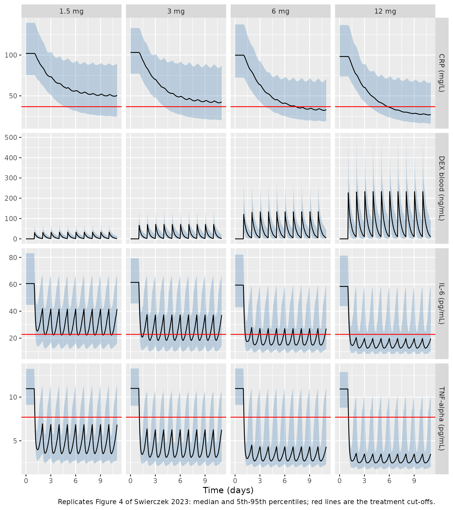
Figure 3 – CRP under the recommended 6 mg regimen
The paper’s Figure 3 overlays published CRP medians and means (Zacharias et al., Kooistra et al.) on the simulated 6 mg regimen; those observed points are not tabulated in the article and are not reproduced here.
sim |>
  dplyr::filter(regimen == "6 mg") |>
  dplyr::group_by(time) |>
  dplyr::summarise(
    Q05 = quantile(crp, 0.05), Q50 = median(crp), Q95 = quantile(crp, 0.95),
    .groups = "drop"
  ) |>
  ggplot(aes(time / 24, Q50)) +
  geom_line(aes(y = Q05), colour = "blue") +
  geom_line(aes(y = Q95), colour = "blue") +
  geom_line() +
  labs(x = "Time (days)", y = "Plasma CRP (mg/L)",
       caption = paste("Replicates Figure 3 of Swierczek 2023: median and",
                       "5th/95th percentiles, 6 mg once daily for 10 days."))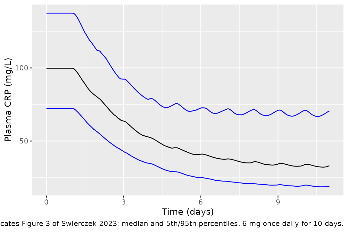
Figure 5 – treatment end points
The Supplement 1 Simulx [ENDPOINT] block scores a
subject as a success when the MAXIMUM biomarker concentration over the
24 h after the assessed dose is at or below the cut-off (TNF-alpha 7.7
pg/mL, IL-6 22.8 pg/mL, CRP 36.7 mg/L); the cumulative end point
requires all three. Day 5 is the 24 h after the fifth dose (t = 120-144
h), day 10 the 24 h after the tenth (t = 240-264 h, the Simulx output
window).
window_max <- function(sim, from, to, day) {
  sim |>
    dplyr::filter(time >= from, time <= to) |>
    dplyr::group_by(id, regimen) |>
    dplyr::summarise(
      TNF = max(tnf) <= 7.7, IL6 = max(il6) <= 22.8, CRP = max(crp) <= 36.7,
      .groups = "drop"
    ) |>
    dplyr::mutate(Cumulative = TNF & IL6 & CRP, day = day)
}
success <- dplyr::bind_rows(
  window_max(sim, 120, 144, "Day 5"),
  window_max(sim, 240, 264, "Day 10")
)

# Figure 5 / Results text: percent of simulated subjects reaching each end point.
published <- tibble::tribble(
  ~day,     ~endpoint, ~`1.5 mg`, ~`3 mg`, ~`6 mg`, ~`12 mg`,
  "Day 5",  "TNF",     55.0,      65.9,    74.8,    81.2,
  "Day 10", "TNF",     55.0,      65.9,    74.8,    81.2,
  "Day 5",  "IL6",     13.0,      26.5,    38.9,    53.1,
  "Day 10", "IL6",     13.0,      26.5,    38.9,    53.1,
  "Day 5",  "CRP",      5.5,      13.5,    21.6,    34.5,
  "Day 10", "CRP",     20.1,      37.3,    53.5,    67.4
) |>
  tidyr::pivot_longer(-c(day, endpoint), names_to = "regimen",
                      values_to = "published_pct")

rates <- success |>
  tidyr::pivot_longer(c(TNF, IL6, CRP, Cumulative), names_to = "endpoint",
                      values_to = "ok") |>
  dplyr::group_by(day, endpoint, regimen) |>
  dplyr::summarise(simulated_pct = 100 * mean(ok), .groups = "drop") |>
  dplyr::mutate(regimen = as.character(regimen))

cmp_rates <- rates |>
  dplyr::inner_join(published, by = c("day", "endpoint", "regimen")) |>
  dplyr::mutate(diff = simulated_pct - published_pct)

cmp_rates |>
  dplyr::arrange(endpoint, day, factor(regimen, levels = levels(regimens$regimen))) |>
  dplyr::rename(
    "Day" = day, "End point" = endpoint, "Regimen" = regimen,
    "Simulated (%)" = simulated_pct, "Published (%)" = published_pct,
    "Difference (points)" = diff
  ) |>
  knitr::kable(digits = 1,
caption = "Percent of subjects reaching each end point (Figure 5).")| Day | End point | Regimen | Simulated (%) | Published (%) | Difference (points) |
|---|---|---|---|---|---|
| Day 10 | CRP | 1.5 mg | 24.0 | 20.1 | 3.9 |
| Day 10 | CRP | 3 mg | 35.0 | 37.3 | -2.3 |
| Day 10 | CRP | 6 mg | 55.0 | 53.5 | 1.5 |
| Day 10 | CRP | 12 mg | 71.5 | 67.4 | 4.1 |
| Day 5 | CRP | 1.5 mg | 7.5 | 5.5 | 2.0 |
| Day 5 | CRP | 3 mg | 9.0 | 13.5 | -4.5 |
| Day 5 | CRP | 6 mg | 24.5 | 21.6 | 2.9 |
| Day 5 | CRP | 12 mg | 36.5 | 34.5 | 2.0 |
| Day 10 | IL6 | 1.5 mg | 16.5 | 13.0 | 3.5 |
| Day 10 | IL6 | 3 mg | 24.5 | 26.5 | -2.0 |
| Day 10 | IL6 | 6 mg | 39.0 | 38.9 | 0.1 |
| Day 10 | IL6 | 12 mg | 58.5 | 53.1 | 5.4 |
| Day 5 | IL6 | 1.5 mg | 16.5 | 13.0 | 3.5 |
| Day 5 | IL6 | 3 mg | 24.5 | 26.5 | -2.0 |
| Day 5 | IL6 | 6 mg | 39.0 | 38.9 | 0.1 |
| Day 5 | IL6 | 12 mg | 58.5 | 53.1 | 5.4 |
| Day 10 | TNF | 1.5 mg | 60.0 | 55.0 | 5.0 |
| Day 10 | TNF | 3 mg | 62.5 | 65.9 | -3.4 |
| Day 10 | TNF | 6 mg | 77.0 | 74.8 | 2.2 |
| Day 10 | TNF | 12 mg | 85.5 | 81.2 | 4.3 |
| Day 5 | TNF | 1.5 mg | 60.0 | 55.0 | 5.0 |
| Day 5 | TNF | 3 mg | 62.5 | 65.9 | -3.4 |
| Day 5 | TNF | 6 mg | 77.5 | 74.8 | 2.7 |
| Day 5 | TNF | 12 mg | 85.5 | 81.2 | 4.3 |
stopifnot(
  # Centre: a wrong IC50, Imax, kout or dose unit shifts every rate by
  # tens of points.
  abs(median(cmp_rates$diff)) < 6,
  # Envelope over 24 rates, each with a Monte-Carlo SE of ~3.5 points at
  # n = 200 per arm; robust to which subjects land in the tails.
  quantile(abs(cmp_rates$diff), 0.9) < 12
)
rates |>
  dplyr::mutate(
    regimen = factor(regimen, levels = levels(regimens$regimen)),
    day = factor(day, levels = c("Day 5", "Day 10")),
    n = simulated_pct / 100 * n_per_arm
  ) |>
  ggplot(aes(endpoint, n, fill = regimen)) +
  geom_col(position = "dodge") +
  facet_wrap(~day) +
  labs(x = "Treatment end point", y = "Subjects reaching end point (of 200)",
       fill = "Regimen",
       caption = "Replicates Figure 5 of Swierczek 2023 (200 rather than 1000 per arm).")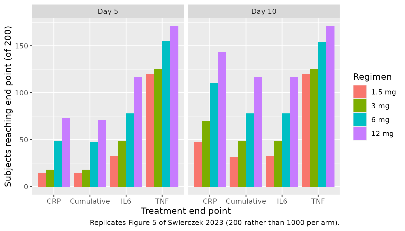
Table S1 – odds ratios against the 6 mg reference (day 10)
odds <- function(p) p / (1 - p)
or_sim <- rates |>
  dplyr::filter(day == "Day 10") |>
  dplyr::group_by(endpoint) |>
  dplyr::mutate(
    p = pmin(pmax(simulated_pct / 100, 0.001), 0.999),
    OR = odds(p) / odds(p[regimen == "6 mg"])
  ) |>
  dplyr::ungroup() |>
  dplyr::filter(regimen != "6 mg") |>
  dplyr::select(endpoint, regimen, OR)

or_pub <- tibble::tribble(
  ~endpoint,    ~regimen,  ~OR_published,
  "CRP",        "1.5 mg",  0.22,
  "CRP",        "3 mg",    0.52,
  "CRP",        "12 mg",   1.8,
  "IL6",        "1.5 mg",  0.24,
  "IL6",        "3 mg",    0.57,
  "IL6",        "12 mg",   1.78,
  "TNF",        "1.5 mg",  0.41,
  "TNF",        "3 mg",    0.65,
  "TNF",        "12 mg",   1.46,
  "Cumulative", "1.5 mg",  0.23,
  "Cumulative", "3 mg",    0.57,
  "Cumulative", "12 mg",   1.78
)

or_cmp <- dplyr::inner_join(or_sim, or_pub, by = c("endpoint", "regimen"))
or_cmp |>
  dplyr::rename("End point" = endpoint, "Regimen vs 6 mg" = regimen,
                "Simulated OR" = OR, "Published OR (Table S1)" = OR_published) |>
knitr::kable(digits = 2, caption = "Odds ratios of reaching the day-10 end point.")| End point | Regimen vs 6 mg | Simulated OR | Published OR (Table S1) |
|---|---|---|---|
| CRP | 1.5 mg | 0.26 | 0.22 |
| CRP | 3 mg | 0.44 | 0.52 |
| CRP | 12 mg | 2.05 | 1.80 |
| Cumulative | 1.5 mg | 0.30 | 0.23 |
| Cumulative | 3 mg | 0.51 | 0.57 |
| Cumulative | 12 mg | 2.20 | 1.78 |
| IL6 | 1.5 mg | 0.31 | 0.24 |
| IL6 | 3 mg | 0.51 | 0.57 |
| IL6 | 12 mg | 2.20 | 1.78 |
| TNF | 1.5 mg | 0.45 | 0.41 |
| TNF | 3 mg | 0.50 | 0.65 |
| TNF | 12 mg | 1.76 | 1.46 |
stopifnot(
  # Centre: the typical simulated OR is within 1.6-fold of Table S1 (log-OR
  # SE is ~0.25 per comparison at n = 200 per arm).
  median(abs(log(or_cmp$OR / or_cmp$OR_published))) < log(1.6),
  # 1.5 mg is far below 6 mg for every end point (published ORs 0.22-0.41,
  # at least 3 SE below 0.8). The 12 mg ORs (1.46-1.8) are too close to 1
  # for a per-row gate at this cohort size.
  all(or_cmp$OR[or_cmp$regimen == "1.5 mg"] < 0.8)
)
PKNCA validation
The paper reports no NCA table. Its Table 1 apparent clearance implies a single-dose AUC0-inf of Dose / (CL/F) = 6 mg / 6.27 L/h = 957 ng*h/mL for the typical 6 mg patient; with log-normal IIV on CL/F, that is also the expected median of the individual AUC0-inf values. The single 6 mg oral dose of the PK study is simulated for 200 patients and analysed with PKNCA.
ev_sd <- tidyr::expand_grid(id = 1:200, time = c(0, 0.25, 0.5, 1, 1.5, 2, 3, 4, 6, 8, 12, 16, 24, 36, 48, 72)) |>
  dplyr::mutate(evid = 0L, amt = 0, cmt = "central") |>
  dplyr::bind_rows(tibble::tibble(id = 1:200, time = 0, evid = 1L, amt = 6, cmt = "depot")) |>
  dplyr::mutate(treatment = "6 mg single dose") |>
  dplyr::arrange(id, time, dplyr::desc(evid))

sim_sd <- rxode2::rxSolve(mod, events = ev_sd, keep = "treatment") |>
  as.data.frame()

sim_nca <- sim_sd |>
  dplyr::filter(!is.na(Cc)) |>
  dplyr::select(id, time, Cc, treatment)
sim_nca <- dplyr::bind_rows(
  sim_nca,
  sim_nca |> dplyr::distinct(id, treatment) |> dplyr::mutate(time = 0, Cc = 0)
) |>
  dplyr::distinct(id, treatment, time, .keep_all = TRUE) |>
  dplyr::arrange(id, treatment, time)

conc_obj <- PKNCA::PKNCAconc(sim_nca, Cc ~ time | treatment + id)
#> Warning in assert_conc(conc, any_missing_conc = any_missing_conc): Negative
#> concentrations found
dose_obj <- PKNCA::PKNCAdose(
  ev_sd |> dplyr::filter(evid == 1) |> dplyr::select(id, time, amt, treatment),
  amt ~ time | treatment + id
)
intervals <- data.frame(start = 0, end = Inf, cmax = TRUE, tmax = TRUE,
                        aucinf.obs = TRUE, half.life = TRUE)
nca_res <- PKNCA::pk.nca(PKNCA::PKNCAdata(conc_obj, dose_obj, intervals = intervals))
#> Warning in assert_conc(conc = conc): Negative concentrations found
#> Warning in assert_conc(conc = conc): Negative concentrations found
#> Warning in assert_conc(conc = conc): Negative concentrations found
#> Warning in assert_conc(conc = conc): Negative concentrations found
#> Warning in assert_conc(conc = conc): Negative concentrations found
#> Warning in assert_conc(conc = conc): Negative concentrations found
#> Warning in log(data$conc): NaNs produced
#> Warning in assert_conc(conc, any_missing_conc = any_missing_conc): Negative
#> concentrations found
#> Warning in log(conc.2/conc.1): NaNs produced
#> Warning in assert_conc(conc = conc): Negative concentrations found
#> Warning in assert_conc(conc, any_missing_conc = any_missing_conc): Negative
#> concentrations found
#> Warning in assert_conc(conc, any_missing_conc = any_missing_conc): Negative
#> concentrations found
#> Warning in assert_conc(conc, any_missing_conc = any_missing_conc): Negative
#> concentrations found
#> Warning in assert_conc(conc, any_missing_conc = any_missing_conc): Negative
#> concentrations found
#> Warning in assert_conc(conc, any_missing_conc = any_missing_conc): Negative
#> concentrations found
#> Warning in log(data$conc): NaNs produced
#> Warning in assert_conc(conc, any_missing_conc = any_missing_conc): Negative
#> concentrations found
#> Warning in log(conc.2/conc.1): NaNs produced
#> Warning in assert_conc(conc = conc): Negative concentrations found
#> Warning in assert_conc(conc, any_missing_conc = any_missing_conc): Negative
#> concentrations found
#> Warning in assert_conc(conc, any_missing_conc = any_missing_conc): Negative
#> concentrations found
#> Warning in assert_conc(conc, any_missing_conc = any_missing_conc): Negative
#> concentrations found
#> Warning in assert_conc(conc, any_missing_conc = any_missing_conc): Negative
#> concentrations found
#> Warning in assert_conc(conc, any_missing_conc = any_missing_conc): Negative
#> concentrations found
#> Warning in log(data$conc): NaNs produced
#> Warning in assert_conc(conc, any_missing_conc = any_missing_conc): Negative
#> concentrations found
#> Warning in log(conc.2/conc.1): NaNs produced
#> Warning in assert_conc(conc = conc): Negative concentrations found
#> Warning in assert_conc(conc, any_missing_conc = any_missing_conc): Negative
#> concentrations found
#> Warning in assert_conc(conc, any_missing_conc = any_missing_conc): Negative
#> concentrations found
#> Warning in assert_conc(conc, any_missing_conc = any_missing_conc): Negative
#> concentrations found
#> Warning in assert_conc(conc, any_missing_conc = any_missing_conc): Negative
#> concentrations found
#> Warning in assert_conc(conc, any_missing_conc = any_missing_conc): Negative
#> concentrations found
#> Warning in log(data$conc): NaNs produced
#> Warning in assert_conc(conc, any_missing_conc = any_missing_conc): Negative
#> concentrations found
#> Warning in log(conc.2/conc.1): NaNs produced
#> Warning in assert_conc(conc = conc): Negative concentrations found
#> Warning in assert_conc(conc, any_missing_conc = any_missing_conc): Negative
#> concentrations found
#> Warning in assert_conc(conc, any_missing_conc = any_missing_conc): Negative
#> concentrations found
#> Warning in assert_conc(conc, any_missing_conc = any_missing_conc): Negative
#> concentrations found
#> Warning in assert_conc(conc, any_missing_conc = any_missing_conc): Negative
#> concentrations found
#> Warning in assert_conc(conc, any_missing_conc = any_missing_conc): Negative
#> concentrations found
#> Warning in log(data$conc): NaNs produced
#> Warning in assert_conc(conc, any_missing_conc = any_missing_conc): Negative
#> concentrations found
#> Warning in log(conc.2/conc.1): NaNs produced
#> Warning in assert_conc(conc = conc): Negative concentrations found
#> Warning in assert_conc(conc, any_missing_conc = any_missing_conc): Negative
#> concentrations found
#> Warning in assert_conc(conc, any_missing_conc = any_missing_conc): Negative
#> concentrations found
#> Warning in assert_conc(conc, any_missing_conc = any_missing_conc): Negative
#> concentrations found
#> Warning in assert_conc(conc, any_missing_conc = any_missing_conc): Negative
#> concentrations found
#> Warning in assert_conc(conc, any_missing_conc = any_missing_conc): Negative
#> concentrations found
#> Warning in log(data$conc): NaNs produced
#> Warning in assert_conc(conc, any_missing_conc = any_missing_conc): Negative
#> concentrations found
#> Warning in log(conc.2/conc.1): NaNs produced

reference <- tibble::tibble(treatment = "6 mg single dose",
                            aucinf.obs = 6 / 6.27 * 1000)
cmp <- nlmixr2lib::ncaComparisonTable(
  simulated = nca_res,
  reference = reference,
  by = "treatment",
  units = c(aucinf.obs = "ng*h/mL"),
  tolerance_pct = 20
)
knitr::kable(cmp, caption = "Simulated median AUC0-inf vs Dose / (CL/F) from Table 1. * differs by >20%.")| NCA parameter | treatment | Reference | Simulated | % diff |
|---|---|---|---|---|
| AUC0-∞ (obs) (ng*h/mL) | 6 mg single dose | 957 | 1020 | +7.0% |
auc_med <- as.data.frame(nca_res) |>
  dplyr::filter(PPTESTCD == "aucinf.obs") |>
  dplyr::pull(PPORRES) |>
  median(na.rm = TRUE)
stopifnot(abs(auc_med / (6 / 6.27 * 1000) - 1) < 0.15)
The day-10 accumulation of DEX is small (Figure 4), matching the paper’s statement that no substantial accumulation occurs even at 12 mg once daily:
acc <- sim |>
  dplyr::filter(regimen == "12 mg", time %in% c(24 + 23, 240 + 23)) |>
  dplyr::group_by(time) |>
  dplyr::summarise(median_trough = median(Cc), .groups = "drop")
knitr::kable(acc, digits = 2, caption = "Median DEX trough (ng/mL), 12 mg once daily, after dose 1 and dose 10.")| time | median_trough |
|---|---|
| 47 | 11.40 |
| 263 | 11.75 |
Assumptions and deviations
-
Drug effect driven by the central concentration.
The printed Eqs 4-5 write the DEX concentration in the inhibition term
as
Cp, the symbol the PK equations use for the peripheral compartment. The Supplement 1 Monolix code that produced every simulation uses the central concentrationCc, and Table 2 defines IC50 as a ‘DEX plasma concentration’; the model follows the code. - IIV magnitudes follow the Supplement 1 code. The Methods say the IIV of IC50 and Imax was ‘set at 20% of the typical value’; Table 2 and the Monolix code give SDs of 0.45 and 0.7 (log scale, IC50) and 0.166 and 0.161 (logit scale, Imax). The tabulated SDs are used as random-effect SDs on the stated log / logit scales, exactly as the Simulx code samples them.
-
Normal lag-time IIV. tlag is normally distributed
in the source (Monolix
distribution=normal), so its random effect is added to tlag in hours. The eta keeps the conventional nameetaltlagbut is not applied on the log scale; a small fraction of simulated subjects get a negative lag. -
Fixed PD parameters. All Table 2 values are encoded
with
fixed(): none was estimated in this paper (they were translated from earlier work, derived as secondary parameters, or set by assumption or trial-and-error simulation). -
IL-6 drives CRP production without baseline
subtraction. Eq 6 uses the absolute IL-6 concentration,
kinCRP * (1 + SIL6onCRP * IL6), so the registered stimulation factorsstim_il6_crpenters with a driver baseline of zero. - No residual error on TNF-alpha, IL-6 or CRP. The PD outputs were never fitted, so the paper has no residual error model for them; they are model states only.
- Figure 3 regimen. The paper’s Figure 3 caption describes intravenous 6 mg doses, while the Simulx code doses all regimens into the oral absorption compartment. The 6 mg oral regimen is used here; with F unknown, an intravenous dose cannot be placed in this apparent-parameter model.
- Cohort size. 200 rather than 1000 simulated subjects per regimen.
- Errata. PubMed lists no erratum or correction linked to this article (checked 2026-10-27).