Indinavir (Csajka 2004)
Source:vignettes/articles/Csajka_2004_indinavir.Rmd
Csajka_2004_indinavir.RmdModel and source
- Citation: Csajka C, Marzolini C, Fattinger K, Decosterd LA, Telenti A, Biollaz J, Buclin T. Population pharmacokinetics of indinavir in patients infected with human immunodeficiency virus. Antimicrob Agents Chemother. 2004;48(9):3226-3232. doi:10.1128/aac.48.9.3226-3232.2004
- Description: One-compartment first-order-absorption population PK model for oral indinavir 800 mg three-times-daily (alone) or 800 mg twice-daily with low-dose ritonavir in HIV-infected adults; concomitant ritonavir, sex, and body weight enter apparent oral clearance as multiplicative covariate effects (Csajka 2004).
- Article: https://doi.org/10.1128/aac.48.9.3226-3232.2004
Population
Csajka 2004 analysed plasma indinavir from 239 HIV-1-infected adults followed at the University Hospital, Lausanne (with samples also analysed in Zurich) over a 40-month period. 569 plasma indinavir samples were collected across 490 visits; the median number of visits per subject was 2 (range 1-8). Seven subjects contributed a full 0.3-8 h time course. Median age was 40.1 years (range 16.3-73.4), median body weight 66.8 kg (41-116), and median height 172 cm (150-194). Females were 70/239 (29.3%) of the cohort, and 92% of subjects with available ethnicity data (122 of 133) were Caucasian. CD4 cell counts ranged 12-1,491 cells/mm^3 (median 433) and HIV viral load 1-750,000 copies/mm^3 (median 400). 62 subjects received indinavir 800 mg three-times-daily without ritonavir; 177 received indinavir 800 mg twice-daily with ritonavir 100 mg twice-daily; 21 patients had been dose-reduced to 400 or 600 mg twice-daily prior to enrollment for tolerability. Baseline demographics are Csajka 2004 Table 1.
The same information is available programmatically via
readModelDb("Csajka_2004_indinavir")$population.
Source trace
The per-parameter origin is also recorded as an in-file comment next
to each ini() entry in
inst/modeldb/specificDrugs/Csajka_2004_indinavir.R. The
table below collects them in one place for review.
| Equation / parameter | Value | Source location |
|---|---|---|
lcl (CL_female, no RTV) |
log(32.4 L/h) | Csajka 2004 Table 3 final-model row “CL_female” |
lvc (V/F) |
log(65.7 L) | Csajka 2004 Table 3 final-model row “V” |
lka (Ka) |
log(1.0 1/h) | Csajka 2004 Table 3 final-model row “Ka” |
lfdepot (F = 1, FIXED) |
log(1) | Csajka 2004 Table 3 footnote h |
e_sex_cl (theta_male on CL/F) |
+0.30 | Csajka 2004 Table 3 final-model row “theta_male” |
e_rtv_cl (theta_RTV on CL/F) |
-0.63 | Csajka 2004 Table 3 final-model row “theta_RTV” |
e_wt_cl (theta_BW on CL/F) |
+0.16 | Csajka 2004 Table 3 final-model row “theta_BW” |
etalcl (IIV CL/F) |
log(1+0.39^2) | Csajka 2004 Table 3 final-model CL/F variability (39% CV) |
etalka (IIV ka) |
log(1+0.67^2) | Csajka 2004 Table 3 final-model Ka variability (67% CV) |
propSd |
0.41 | Csajka 2004 Table 3 final-model sigma (CV%) 41% |
addSd |
0.670 mg/L | Csajka 2004 Table 3 final-model sigma (SD; ug/L) 670 |
| CL/F equation | n/a | Csajka 2004 Table 3 footnote a; Methods, model-building text |
| 1-cmt + first-order absorption | n/a | Csajka 2004 Results, “Population pharmacokinetic analysis” |
Virtual cohort
Csajka 2004’s individual concentration data are not publicly available. The cohort below approximates the published demographics (Csajka 2004 Table 1) and stratifies by the two clinically relevant covariate contrasts: sex (male / female) and concomitant ritonavir (with / without). Body weight is drawn from a log-normal distribution targeting the published median 66.8 kg and a 41-116 kg span (sd of log-WT chosen so that ~95% of weights fall in 45-100 kg).
set.seed(20040901L)
n_per_arm <- 60L

draw_wt <- function(n) {
  # Log-normal weight: median 66.8 kg, ~95% in 45-100 kg.
  pmin(pmax(round(rlnorm(n, meanlog = log(66.8), sdlog = 0.18), 1), 41), 116)
}

make_arm <- function(id_offset, label, n, regimen_label, sexf, conmed_rtv, dose_mg, tau) {
  # Steady-state dosing achieved by a single dose with `ss = 1` and an
  # interval `ii = tau`; rxSolve then evaluates the system as if the
  # subject has been on the regimen for many intervals. Observations
  # are taken over a single dosing interval starting at the SS dose.
  obs_times <- seq(0, tau, by = 0.2)
  wts       <- draw_wt(n)
  ids       <- id_offset + seq_len(n)

  doses <- tibble::tibble(
    id   = ids,
    time = 0,
    evid = 1L,
    amt  = dose_mg,
    cmt  = "depot",
    ss   = 1L,
    ii   = tau
  )

  obs <- expand.grid(id = ids, time = obs_times, KEEP.OUT.ATTRS = FALSE) |>
    dplyr::mutate(evid = 0L, amt = 0, cmt = NA_character_, ss = 0L, ii = 0)

  covars <- tibble::tibble(
    id         = ids,
    WT         = wts,
    SEXF       = sexf,
    CONMED_RTV = conmed_rtv
  )

  dplyr::bind_rows(doses, obs) |>
    dplyr::arrange(id, time, dplyr::desc(evid)) |>
    dplyr::left_join(covars, by = "id") |>
    dplyr::mutate(
      arm       = label,
      regimen   = regimen_label,
      dose_mg   = dose_mg,
      tau_h     = tau
    )
}

events <- dplyr::bind_rows(
  # Male, no ritonavir, 800 mg t.i.d. (tau = 8 h)
  make_arm(  0L, "Male no-RTV",     n_per_arm, "800 mg q8h",
           sexf = 0L, conmed_rtv = 0L, dose_mg = 800, tau = 8),
  # Female, no ritonavir, 800 mg t.i.d.
  make_arm(1000L, "Female no-RTV",  n_per_arm, "800 mg q8h",
           sexf = 1L, conmed_rtv = 0L, dose_mg = 800, tau = 8),
  # Male, ritonavir, 800 mg b.i.d. (tau = 12 h)
  make_arm(2000L, "Male + RTV",     n_per_arm, "800/100 mg q12h",
           sexf = 0L, conmed_rtv = 1L, dose_mg = 800, tau = 12),
  # Female, ritonavir, 800 mg b.i.d.
  make_arm(3000L, "Female + RTV",   n_per_arm, "800/100 mg q12h",
           sexf = 1L, conmed_rtv = 1L, dose_mg = 800, tau = 12)
)

stopifnot(!anyDuplicated(unique(events[, c("id", "time", "evid")])))
Simulation
Stochastic VPC simulation using the packaged model with between-subject variability on CL/F and ka.
mod <- readModelDb("Csajka_2004_indinavir")()

sim <- rxode2::rxSolve(
  mod,
  events = events,
  keep = c("arm", "regimen", "dose_mg", "tau_h", "WT", "SEXF", "CONMED_RTV")
) |>
  as.data.frame() |>
  dplyr::as_tibble()
For deterministic typical-value replication we also simulate a
single-subject-per-arm cohort at the 70 kg reference weight, with the
random effects zeroed out (rxode2::zeroRe); these four
profiles reproduce the typical-value steady-state predictions published
in Csajka 2004’s “Dosage regimen adaptation” paragraph.
make_typ_arm <- function(id, label, regimen_label, sexf, conmed_rtv,
                         dose_mg, tau) {
  obs_times <- seq(0, tau, by = 0.1)
  dose_row <- tibble::tibble(
    id   = id, time = 0,    evid = 1L, amt = dose_mg,
    cmt  = "depot", ss = 1L, ii = tau
  )
  obs_rows <- tibble::tibble(
    id   = id, time = obs_times, evid = 0L, amt = 0,
    cmt  = NA_character_, ss = 0L, ii = 0
  )
  dplyr::bind_rows(dose_row, obs_rows) |>
    dplyr::mutate(
      WT         = 70,
      SEXF       = sexf,
      CONMED_RTV = conmed_rtv,
      arm        = label,
      regimen    = regimen_label,
      dose_mg    = dose_mg,
      tau_h      = tau
    )
}

events_typ <- dplyr::bind_rows(
  make_typ_arm(1L, "Male no-RTV",    "800 mg q8h",
               sexf = 0L, conmed_rtv = 0L, dose_mg = 800, tau = 8),
  make_typ_arm(2L, "Female no-RTV",  "800 mg q8h",
               sexf = 1L, conmed_rtv = 0L, dose_mg = 800, tau = 8),
  make_typ_arm(3L, "Male + RTV",     "800/100 mg q12h",
               sexf = 0L, conmed_rtv = 1L, dose_mg = 800, tau = 12),
  make_typ_arm(4L, "Female + RTV",   "800/100 mg q12h",
               sexf = 1L, conmed_rtv = 1L, dose_mg = 800, tau = 12)
)

mod_typical <- rxode2::zeroRe(mod)
sim_typical <- rxode2::rxSolve(
  mod_typical,
  events = events_typ,
  keep   = c("arm", "regimen", "dose_mg", "tau_h", "WT", "SEXF", "CONMED_RTV")
) |>
  as.data.frame() |>
  dplyr::as_tibble()
#> ℹ omega/sigma items treated as zero: 'etalcl', 'etalka'
#> Warning: multi-subject simulation without without 'omega'
Replicate published predictions
Csajka 2004 page 3229 (“Dosage regimen adaptation”) gives a-priori typical-value steady-state C_av and C_min for a 70 kg male and a 70 kg female under each of the two standard regimens. The figure below shows the simulated steady-state profile for each arm, and the table that follows compares simulated values against the paper’s text.
sim_typical |>
  dplyr::filter(!is.na(Cc)) |>
  ggplot(aes(time, Cc * 1000, colour = arm)) +
  geom_line(alpha = 0.8) +
  facet_wrap(~regimen, scales = "free_x") +
  labs(
    x = "Time since last (steady-state) dose (h)",
    y = "Indinavir plasma concentration (ug/L)",
    colour = "Stratum",
    title = "Csajka 2004 typical-value steady-state profiles"
  )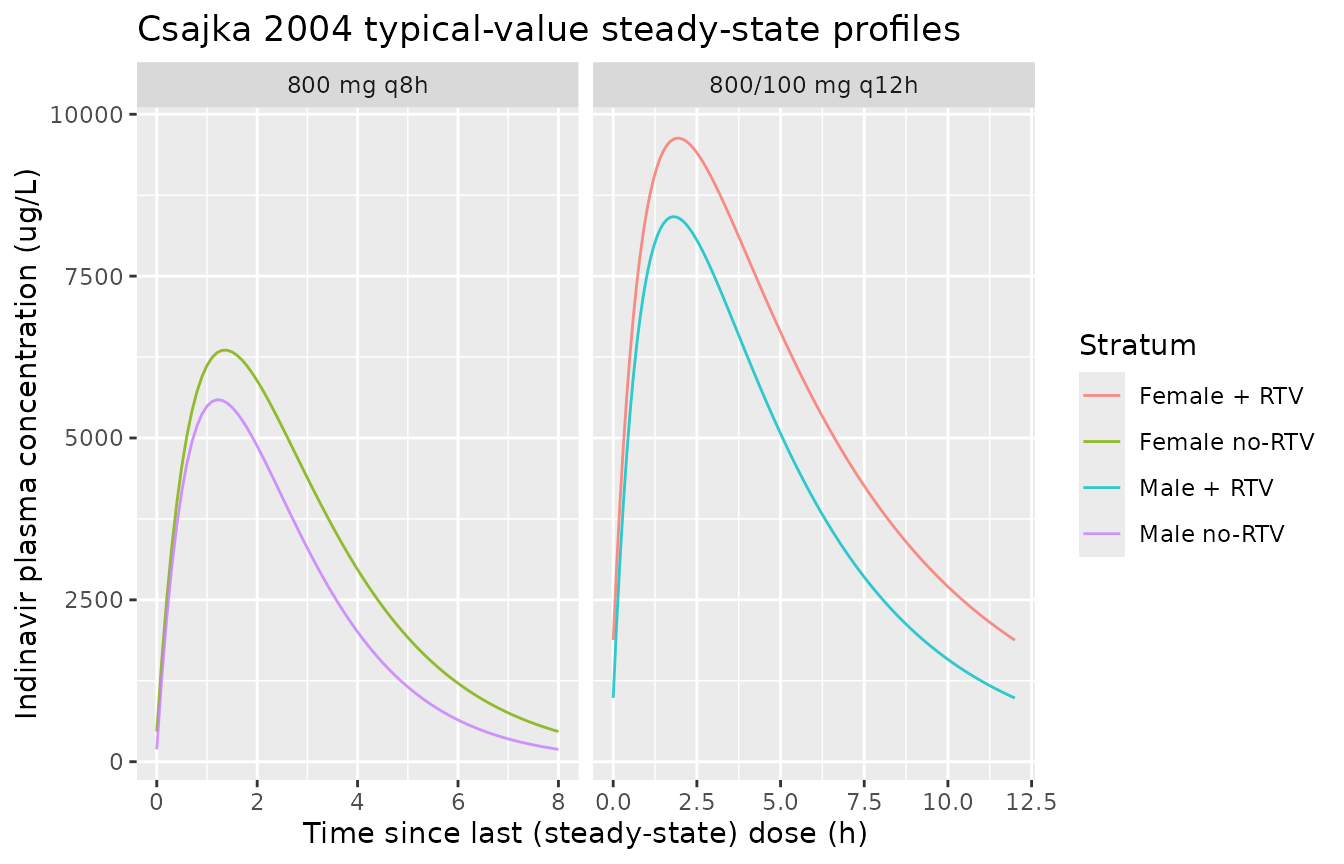
Typical-value steady-state plasma indinavir over one dosing interval for the four arms (70 kg reference subject).
sim |>
  dplyr::filter(!is.na(Cc)) |>
  dplyr::group_by(arm, regimen, time) |>
  dplyr::summarise(
    Q05 = stats::quantile(Cc, 0.05, na.rm = TRUE),
    Q50 = stats::quantile(Cc, 0.50, na.rm = TRUE),
    Q95 = stats::quantile(Cc, 0.95, na.rm = TRUE),
    .groups = "drop"
  ) |>
  ggplot(aes(time, Q50 * 1000, colour = arm, fill = arm)) +
  geom_ribbon(aes(ymin = Q05 * 1000, ymax = Q95 * 1000), alpha = 0.2, colour = NA) +
  geom_line() +
  facet_wrap(~regimen, scales = "free_x") +
  scale_y_log10() +
  labs(
    x = "Time since last (steady-state) dose (h)",
    y = "Indinavir plasma concentration (ug/L)",
    colour = "Stratum", fill = "Stratum",
    title = "Csajka 2004 stochastic VPC (5/50/95)"
  )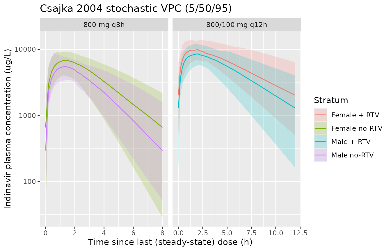
Stochastic 5/50/95 prediction interval over one steady-state dosing interval.
PKNCA validation
Steady-state NCA (AUC0-tau, Cmax, Cmin, Cav) on the typical-value profiles, by stratum. PKNCA is used (no inline trapezoidal calculations).
# The typical-value cohort has one 70 kg subject per arm. The simulated
# events are anchored at t = 0 (the steady-state dose), so the PKNCA AUC
# interval is [0, tau] for each arm.
nca_typical_conc <- sim_typical |>
  dplyr::filter(!is.na(Cc)) |>
  dplyr::select(id, time, Cc, arm)

nca_typical_dose <- events_typ |>
  dplyr::filter(evid == 1L) |>
  dplyr::select(id, time, amt, arm)

conc_obj <- PKNCA::PKNCAconc(nca_typical_conc, Cc ~ time | arm + id,
                             concu = "mg/L", timeu = "hr")
dose_obj <- PKNCA::PKNCAdose(nca_typical_dose, amt ~ time | arm + id,
                             doseu = "mg")

tau_table <- events_typ |>
  dplyr::distinct(arm, tau_h)

# PKNCA's intervals frame is per-group when the formula has a treatment
# grouping; one row per arm with the [0, tau] window keeps the SS NCA
# scoped to a single dosing interval.
intervals_per_arm <- tau_table |>
  dplyr::transmute(
    arm     = arm,
    start   = 0,
    end     = tau_h,
    cmax    = TRUE,
    tmax    = TRUE,
    cmin    = TRUE,
    auclast = TRUE,
    cav     = TRUE,
    ctrough = TRUE
  ) |>
  as.data.frame()

nca_data <- PKNCA::PKNCAdata(conc_obj, dose_obj, intervals = intervals_per_arm)
nca_res  <- PKNCA::pk.nca(nca_data)
nca_summary <- as.data.frame(nca_res$result)

# Display Cav, Cmin, Cmax in ug/L (paper convention; model output is mg/L)
nca_table <- nca_summary |>
  dplyr::filter(PPTESTCD %in% c("cav", "cmin", "cmax", "auclast")) |>
  dplyr::select(arm, PPTESTCD, PPORRES) |>
  tidyr::pivot_wider(names_from = PPTESTCD, values_from = PPORRES) |>
  dplyr::mutate(
    cav_ugL    = cav  * 1000,
    cmin_ugL   = cmin * 1000,
    cmax_ugL   = cmax * 1000,
    aucss_mghL = auclast
  ) |>
  dplyr::select(arm, cav_ugL, cmin_ugL, cmax_ugL, aucss_mghL)

knitr::kable(
  nca_table,
  digits  = c(0, 0, 0, 0, 2),
  caption = "Simulated typical-value steady-state NCA per stratum (PKNCA on the 70 kg reference subject)."
)| arm | cav_ugL | cmin_ugL | cmax_ugL | aucss_mghL |
|---|---|---|---|---|
| Male no-RTV | 2373 | 191 | 5591 | 18.98 |
| Female no-RTV | 3085 | 466 | 6356 | 24.68 |
| Male + RTV | 4277 | 984 | 8419 | 51.32 |
| Female + RTV | 5560 | 1878 | 9631 | 66.72 |
Comparison against Csajka 2004 page 3229
Csajka 2004 explicitly reports a-priori typical-value C_av and C_min for a 70 kg male and a 70 kg female under each regimen (“Dosage regimen adaptation” paragraph, page 3229):
| Stratum | C_av (ug/L) Csajka | C_av (ug/L) sim | C_min (ug/L) Csajka | C_min (ug/L) sim |
|---|---|---|---|---|
| Male, no RTV (800 mg q8h) | 2,391 | 2373 | 193 | 191 |
| Female, no RTV (800 mg q8h) | 3,086 | 3085 | 466 | 466 |
| Male + RTV (800/100 mg q12h) | 4,246 | 4277 | 964 | 984 |
| Female + RTV (800/100 mg q12h) | 5,510 | 5560 | 1,839 | 1878 |
The simulated C_av and C_min match the paper’s reported typical-value predictions within rounding (the small residual gap stems from Csajka rounding the male-without-RTV CL/F to 42.0 L/h vs the model’s exact 32.4 * 1.30 = 42.12 L/h, and the corresponding rounding when the ritonavir multiplier (1 - 0.63) = 0.37 is applied).
Csajka 2004 also reports an absorption half-life of 41 minutes
(Results paragraph 1); the model gives
log(2)/1.0 = 0.693 h = 41.6 min, consistent with the paper.
Elimination half-life increases from 1.4 h (female, no RTV) to 3.8 h
(female + RTV) per the Discussion; the model gives
log(2) / (32.4 / 65.7) = 1.40 h and
log(2) / (32.4 * 0.37 / 65.7) = 3.80 h, matching to two
significant figures.
Assumptions and deviations
-
Sex-encoding inversion. Csajka 2004 Table 3 codes
sex as a male indicator (sex = 1 if male, with female as the reference
category for CL_female = 32.4 L/h). The canonical SEXF (1 = female)
inverts the values; the model applies the +30% male effect via
(1 + e_sex_cl * (1 - SEXF))so the female reference (SEXF = 1) reproduces 32.4 L/h and males (SEXF = 0) reproduce 42.1 L/h. - Concentration units. Csajka 2004 reports concentrations in ug/L; the model uses mg/L (1 mg/L = 1000 ug/L). The 670 ug/L additive residual SD becomes 0.670 mg/L on the model scale, and the figures / table convert simulated mg/L back to ug/L for easy comparison.
- Body weight distribution. The paper reports median 66.8 kg (range 41-116) but does not publish the full BW distribution; the virtual cohort draws WT log-normally targeting the median and a 95% span of 45-100 kg.
- Reduced-dose subgroup not simulated. Csajka 2004 enrolled 21 patients who had already been dose-reduced to 400 or 600 mg twice-daily for tolerability. They are part of the population-PK fit but are not separately tabulated; the virtual cohort uses the protocol-standard 800 mg dose and a single dosing interval per arm rather than a heterogeneous mix.
- HIV-disease covariates omitted from the final model. Ethnicity (Caucasian / Black / Asian / Hispanic indicators), height, age, CD4 count, viral load, CYP3A4 inducers, CYP3A4 inhibitors, and efavirenz / other reverse transcriptase inhibitors were tested as covariates in the screening step (Csajka 2004 Table 2) but did not meet the OFV criterion for inclusion in the final model. The packaged model carries only the three covariates retained in Table 3 (sex, concomitant ritonavir, body weight).
- No interoccasion variability. Csajka 2004 notes a “high residual variability mainly reflecting an interoccasion variability” in the Discussion but does not separately estimate IOV; the model treats all intra-patient variability as combined proportional + additive residual error per Table 3.