Meropenem in neonatal and paediatric ECMO and CRRT (Pokorna 2024)
Source:vignettes/articles/Pokorna_2024_meropenem.Rmd
Pokorna_2024_meropenem.RmdModel and source
mod <- rxode2::rxode2(readModelDb("Pokorna_2024_meropenem"))
#> ℹ parameter labels from comments will be replaced by 'label()'- Model: One-compartment IV population PK model for meropenem in 45 critically ill neonates and children aged 0-5 years, 38 of them on extracorporeal membrane oxygenation (ECMO) and 31 on continuous renal replacement therapy (CRRT) (Pokorna 2024). Clearance and volume of distribution both scale linearly with body weight normalised to the cohort median of 7.88 kg (CL 1.09 L/h, V 3.98 L). CRRT running at the time of the sample raises the volume of distribution by a factor of (1 + 1.04), about two-fold; ECMO had no retained effect. Log-normal interindividual variability on CL and V, and a proportional residual error.
- Citation: Pokorna P, Michalickova D, Tibboel D, Berner J. Meropenem Disposition in Neonatal and Pediatric Extracorporeal Membrane Oxygenation and Continuous Renal Replacement Therapy. Antibiotics (Basel). 2024;13(5):419. doi:10.3390/antibiotics13050419
- Article: https://doi.org/10.3390/antibiotics13050419 (open access)
Pokorna 2024 pooled routine therapeutic drug monitoring (TDM) samples from critically ill neonates and children treated with meropenem, most of them on extracorporeal membrane oxygenation (ECMO), and fitted a one-compartment model in NONMEM 7.3. Body weight scales clearance and volume linearly; continuous renal replacement therapy (CRRT) running at the time of sampling roughly doubles the volume of distribution. ECMO itself had no retained effect.
Population
The study was retrospective and covered 1 January 2018 to 31 December 2020 in the paediatric intensive care unit and ECMO centre of Astrid Lindgren Children’s Hospital (Karolinska University Hospital, Stockholm). It included 45 patients aged 0-5 years with at least two meropenem concentrations: 27 neonates (60%), 4 infants (9%) and 14 children (31%), 23 male and 22 female (Table 1). Body weight was median 7.88 kg (interquartile range 3.62-11.97) and postnatal age at the start of therapy median 3 days (IQR 0-465). 38 patients were on ECMO (31 veno-arterial, 7 veno-venous) and 31 on CRRT (CVVHD or CVVHDF), 19 of them for fluid overload and 12 for acute kidney injury. The 152 plasma concentrations ranged from 0.68 to 75 mg/L; 94 were drawn on ECMO and 91 during CRRT (Results 2.1, Table S1).
Off ECMO, meropenem was given at 20-40 mg/kg over 15-30 min two to four times a day. On ECMO it was given as a 20 mg/kg loading dose followed by a continuous infusion of 30-80 mg/kg/day (0-2 months) or 60-120 mg/kg/day (3 months to 12 years), titrated toward 20-40 mg/L (Methods 4.2).
The same information is available programmatically via
readModelDb("Pokorna_2024_meropenem") and the model’s
population metadata.
Source trace
| Element | Value | Source location |
|---|---|---|
| Structure | one compartment, first-order elimination, IV infusion | Results 2.2; Methods 4.4 |
| CL equation | CL = CLp * (BW/7.88) |
Table 2 |
| V equation | Vd = Vp * (BW/7.88) * (1 + thetaCRRT)^CRRT_on |
Table 2 |
lcl |
log(1.09) L/h at 7.88 kg | Table 2 (RSE 8%); Abstract; Results 2.2 |
lvc |
log(3.98) L at 7.88 kg, off CRRT | Table 2 (RSE 14%); Abstract; Results 2.2 |
e_crrt_vc |
1.04 | Table 2 (RSE 76%) |
etalcl |
omega^2 = 0.0887 | Table 2 ‘CL (%)’ row (RSE 48%) |
etalvc |
omega^2 = 0.916 | Table 2 ‘Vd (%)’ row (RSE 68%) |
propSd |
sqrt(0.17) = 0.412 | Table 2 ‘Proportional’ row (RSE 17%) |
RRT_CRRT_ACTIVE |
CRRT on (1) / off (0) at the sample | Table 2 footnote ‘CRRT_on’; Results 2.1; Table S1 |
| Reference weight | 7.88 kg (cohort median) | Table 1; Table 2; Results 2.2 |
Typical-value checks
The Discussion reports the weight-normalised typical values as 0.138
L/h/kg for CL and 0.51 L/kg for V. Both follow from Table 2 at the
reference weight, and the CRRT factor is 1 + 1.04 = 2.04,
the “approximately two times” increase stated in Results 2.2.
th <- mod$theta
cl_typ <- exp(th[["lcl"]])
v_typ <- exp(th[["lvc"]])
crrt_factor <- 1 + th[["e_crrt_vc"]]

typ <- data.frame(
  Quantity = c("CL / BW (L/h/kg)", "V / BW off CRRT (L/kg)", "V on / V off CRRT", "t1/2 off CRRT (h)", "t1/2 on CRRT (h)"),
  Model = c(cl_typ / 7.88, v_typ / 7.88, crrt_factor, log(2) * v_typ / cl_typ, log(2) * v_typ * crrt_factor / cl_typ),
  Paper = c("0.138 (Discussion)", "0.51 (Discussion)", "approx. 2 (Results 2.2)", "not reported", "not reported")
)
knitr::kable(typ, digits = 3)| Quantity | Model | Paper |
|---|---|---|
| CL / BW (L/h/kg) | 0.138 | 0.138 (Discussion) |
| V / BW off CRRT (L/kg) | 0.505 | 0.51 (Discussion) |
| V on / V off CRRT | 2.040 | approx. 2 (Results 2.2) |
| t1/2 off CRRT (h) | 2.531 | not reported |
| t1/2 on CRRT (h) | 5.163 | not reported |
Virtual cohort under the ECMO dosing protocol
The cohort below mimics the patients who contributed most of the samples: a 20 mg/kg loading dose over 30 min followed by a continuous infusion of 60 mg/kg/day, simulated for 7 days. Body weight is drawn from a split log-normal distribution that reproduces the Table 1 median and IQR, truncated to 2-25 kg (0-5 years). Because 91 of the 152 samples were drawn during CRRT, 60% of the virtual subjects are on CRRT throughout. Concentrations include the residual error.
set.seed(20240419)
n_sub <- 200
z <- rnorm(n_sub)
# Split log-normal: the lower half is spread to the 25th percentile (3.62 kg),
# the upper half to the 75th (11.97 kg); qnorm(0.75) = 0.674.
log_wt <- log(7.88) + ifelse(z < 0, z * log(7.88 / 3.62), z * log(11.97 / 7.88)) / qnorm(0.75)
cohort <- data.frame(
  id = seq_len(n_sub),
  WT = pmin(pmax(exp(log_wt), 2), 25),
  RRT_CRRT_ACTIVE = rbinom(n_sub, 1, 0.6)
)

load_amt <- 20 * cohort$WT
cont_amt <- 60 * cohort$WT * 7
ev_cohort <- bind_rows(
  data.frame(id = cohort$id, time = 0, amt = load_amt, rate = load_amt / 0.5, evid = 1),
  data.frame(id = cohort$id, time = 0.5, amt = cont_amt, rate = cont_amt / 168, evid = 1),
  tidyr::expand_grid(id = cohort$id, time = c(seq(0, 24, by = 1), seq(26, 168, by = 2))) |>
    mutate(amt = NA_real_, rate = NA_real_, evid = 0)
) |>
  mutate(cmt = "central") |>
  left_join(cohort, by = "id") |>
  arrange(id, time, desc(evid))

rxode2::rxSetSeed(20240419)
sim_cohort <- rxode2::rxSolve(mod, events = ev_cohort, returnType = "data.frame")

vpc <- sim_cohort |>
  filter(!is.na(sim)) |>
  mutate(CRRT = ifelse(RRT_CRRT_ACTIVE == 1, "CRRT on", "CRRT off")) |>
  group_by(time, CRRT) |>
  summarise(
    p05 = quantile(sim, 0.05), p50 = median(sim), p95 = quantile(sim, 0.95),
    .groups = "drop"
  )

ggplot(vpc, aes(time, p50, colour = CRRT, fill = CRRT)) +
  geom_ribbon(aes(ymin = p05, ymax = p95), alpha = 0.2, colour = NA) +
  geom_line() +
  labs(
    x = "Time after first dose (h)", y = "Meropenem concentration (mg/L)",
    colour = NULL, fill = NULL,
    caption = "Simulated median and 90% interval; compare with Figure 1 of Pokorna 2024."
  ) +
  theme_bw()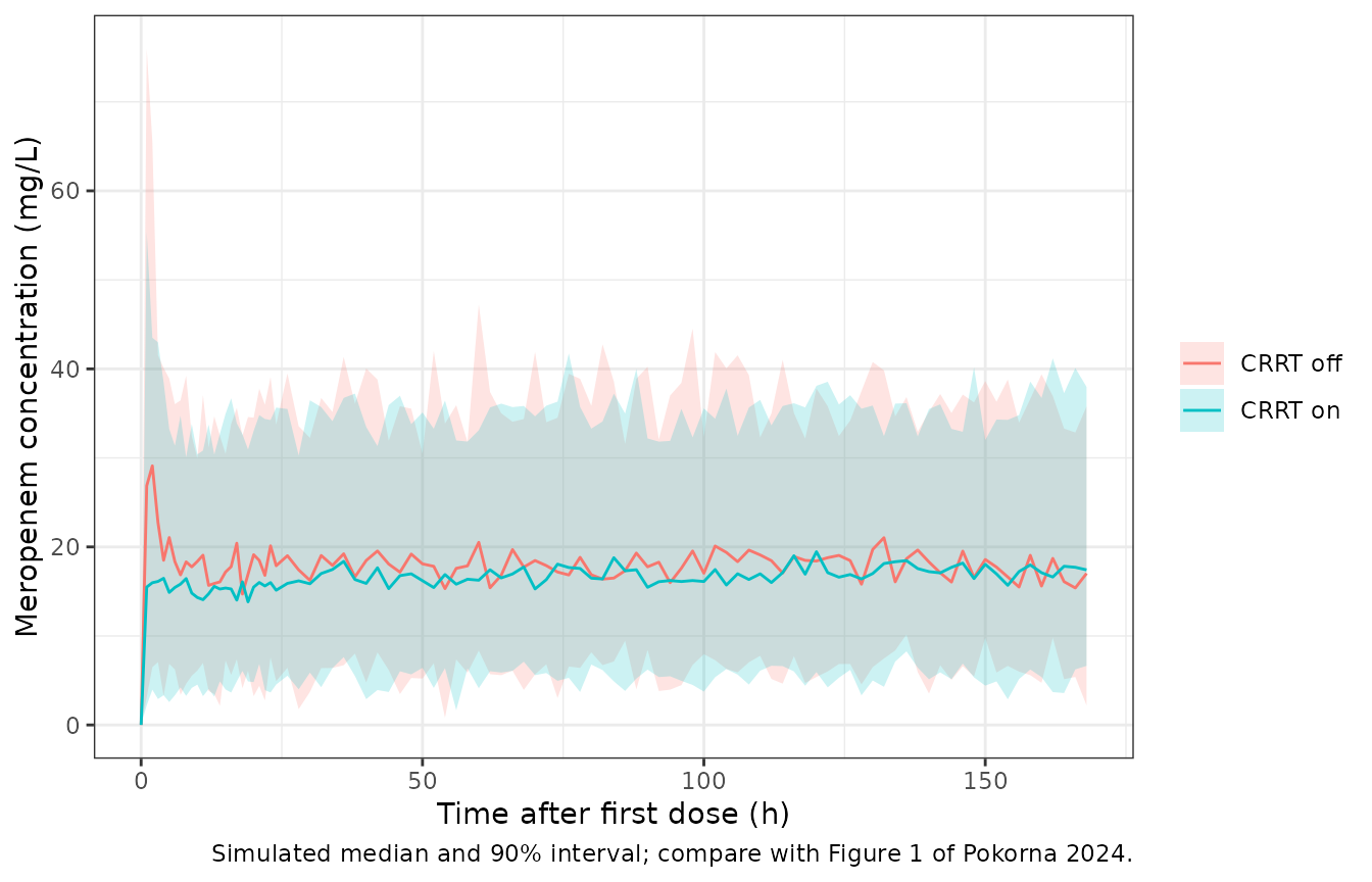
Figure 1 of the paper shows observed concentrations mostly between
about 5 and 40 mg/L across the whole course, under the 20-40 mg/L
titration target. The steady-state concentration of a continuous
infusion is rate / CL, which does not depend on V, so the
two CRRT arms converge once steady state is reached; the CRRT arm
approaches it more slowly because its V is twice as large.
css <- sim_cohort |>
  filter(time == 168) |>
  mutate(css_expected = (60 * WT / 24) / (cl_typ * WT / 7.88))
# The typical-value steady state for 60 mg/kg/day is 60 * 7.88 / 24 / 1.09
# = 18.1 mg/L at any weight (CL and the dose both scale with WT). The cohort
# median of the individual predictions sits on it; the residual-error
# concentrations spread around it.
stopifnot(
  abs(median(css$css_expected) - 18.07) < 0.05,
  abs(median(css$ipredSim) / 18.07 - 1) < 0.15,
  median(css$sim) > 5, median(css$sim) < 40
)
PKNCA validation
The paper reports no NCA. The check below runs PKNCA on the last
dosing interval of 20 mg/kg infused over 30 min every 8 h for a 7.88 kg
patient, at steady state, and compares the result against the
closed-form values implied by the Table 2 typical values
(AUCtau = dose / CL, terminal
t1/2 = log(2) * V / CL).
dose_mg <- 20 * 7.88
ev_nca <- bind_rows(
  tidyr::expand_grid(id = 1:2, time = 0) |>
    mutate(amt = dose_mg, rate = dose_mg / 0.5, ii = 8, ss = 1, evid = 1),
  tidyr::expand_grid(id = 1:2, time = seq(0, 8, by = 0.05)) |>
    mutate(amt = NA_real_, rate = NA_real_, ii = NA_real_, ss = NA_real_, evid = 0)
) |>
  mutate(
    cmt = "central", WT = 7.88, RRT_CRRT_ACTIVE = id - 1,
    treatment = ifelse(RRT_CRRT_ACTIVE == 1, "CRRT on", "CRRT off")
  ) |>
  arrange(id, time, desc(evid))

sim_nca <- rxode2::rxSolve(
  rxode2::zeroRe(mod),
  events = ev_nca, keep = "treatment", returnType = "data.frame",
  rtol = 1e-10, atol = 1e-12, ssRtol = 1e-10, ssAtol = 1e-12,
  maxsteps = 1e6
)
#> ℹ omega/sigma items treated as zero: 'etalcl', 'etalvc'
#> Warning: multi-subject simulation without without 'omega'

# A subject that fails to solve comes back NA; stop rather than drop it.
stopifnot(!anyNA(sim_nca$Cc))
conc_df <- sim_nca |>
  filter(!is.na(Cc)) |>
  select(id, time, Cc, treatment)
dose_df <- ev_nca |>
  filter(evid == 1) |>
  select(id, time, amt, treatment)

conc_obj <- PKNCA::PKNCAconc(conc_df, Cc ~ time | treatment + id, concu = "mg/L", timeu = "h")
dose_obj <- PKNCA::PKNCAdose(dose_df, amt ~ time | treatment + id, doseu = "mg")
intervals <- data.frame(
  start = 0, end = 8,
  cmax = TRUE, cmin = TRUE, auclast = TRUE, half.life = TRUE
)
nca <- PKNCA::pk.nca(PKNCA::PKNCAdata(conc_obj, dose_obj, intervals = intervals))

reference <- data.frame(
  treatment = c("CRRT off", "CRRT on"),
  auclast = dose_mg / cl_typ,
  half.life = log(2) * v_typ * c(1, crrt_factor) / cl_typ
)
cmp <- nlmixr2lib::ncaComparisonTable(
  nca, reference,
  by = "treatment", params = c("auclast", "half.life"),
  units = c(auclast = "mg*h/L", half.life = "h")
)
knitr::kable(cmp, caption = "PKNCA at steady state versus the Table 2 closed form (typical 7.88 kg patient).")| NCA parameter | treatment | Reference | Simulated | % diff |
|---|---|---|---|---|
| AUClast (mg*h/L) | CRRT off | 145 | 145 | -0.0% |
| AUClast (mg*h/L) | CRRT on | 145 | 145 | -0.0% |
| t½ (h) | CRRT off | 2.53 | 2.53 | +0.0% |
| t½ (h) | CRRT on | 5.16 | 5.16 | +0.0% |
chk_nca <- as.data.frame(nca$result) |>
  filter(PPTESTCD %in% c("auclast", "half.life")) |>
  select(treatment, PPTESTCD, PPORRES) |>
  inner_join(
    tidyr::pivot_longer(reference, -treatment, names_to = "PPTESTCD", values_to = "expected"),
    by = c("treatment", "PPTESTCD")
  ) |>
  mutate(pct = 100 * (PPORRES / expected - 1))
# Same parameters on both sides: the only difference is the trapezoid and
# the log-linear lambda_z fit on a 0.05 h grid, well under 1%.
stopifnot(nrow(chk_nca) == 4L, all(abs(chk_nca$pct) < 1))
Replicating Table 3 (probability of target attainment)
Table 3 gives the probability of target attainment (PTA) for 40% and 100% of the dosing interval with the concentration above the MIC, for a 7.88 kg patient on and off CRRT, under six regimens simulated for 7 days. The simulation below uses 200 subjects per regimen and CRRT arm, evaluates the time above the MIC on the individual predictions over the last 8 h of day 7, and treats total concentration as free (meropenem protein binding is about 2%). Continuous infusions start without a loading dose.
regimens <- tibble::tribble(
  ~regimen, ~mg_per_kg, ~duration, ~tau,
  "20 mg/kg 30 min q8h", 20, 0.5, 8,
  "20 mg/kg 3 h q8h", 20, 3, 8,
  "40 mg/kg 30 min q8h", 40, 0.5, 8,
  "40 mg/kg 3 h q8h", 40, 3, 8,
  "60 mg/kg/day cont.", 60, 168, 168,
  "120 mg/kg/day cont.", 120, 168, 168
)
arms <- tidyr::expand_grid(reg = seq_len(nrow(regimens)), CRRT = 0:1) |>
  mutate(arm = row_number())
n_arm <- 200
wt_pta <- 7.88

make_arm <- function(a) {
  rg <- regimens[arms$reg[a], ]
  ids <- (a - 1) * n_arm + seq_len(n_arm)
  dose_amt <- if (rg$tau == 168) rg$mg_per_kg * wt_pta * 7 else rg$mg_per_kg * wt_pta
  doses <- tidyr::expand_grid(id = ids, time = seq(0, 168 - rg$tau, by = rg$tau)) |>
    mutate(amt = dose_amt, rate = dose_amt / rg$duration, evid = 1)
  obs <- tidyr::expand_grid(id = ids, time = seq(160, 168, by = 0.1)) |>
    mutate(amt = NA_real_, rate = NA_real_, evid = 0)
  bind_rows(doses, obs) |>
    mutate(cmt = "central", WT = wt_pta, RRT_CRRT_ACTIVE = arms$CRRT[a], arm = a)
}
ev_pta <- bind_rows(lapply(arms$arm, make_arm)) |> arrange(id, time, desc(evid))

rxode2::rxSetSeed(419)
sim_pta <- rxode2::rxSolve(mod, events = ev_pta, keep = "arm", returnType = "data.frame")

mics <- c(0.5, 1, 2, 4, 8, 16)
ft <- sim_pta |>
  filter(time < 168) |>
  tidyr::crossing(MIC = mics) |>
  group_by(arm, id, MIC) |>
  summarise(ft = mean(Cc > MIC), .groups = "drop")
pta_sim <- ft |>
  group_by(arm, MIC) |>
  summarise(`40` = 100 * mean(ft >= 0.4), `100` = 100 * mean(ft >= 1), .groups = "drop") |>
  tidyr::pivot_longer(c(`40`, `100`), names_to = "target", values_to = "Simulated") |>
  left_join(arms, by = "arm") |>
  mutate(regimen = regimens$regimen[reg]) |>
  select(regimen, CRRT, target, MIC, Simulated)
# Table 3 of Pokorna 2024 (7.88 kg), columns in the order of `arms`:
# regimen 1-6, CRRT = 0 then 1 within each regimen.
paper_40 <- rbind(
  c(93, 98, 98, 99, 95, 98, 98, 99, 100, 100, 100, 100),
  c(91, 97, 97, 99, 93, 98, 98, 99, 100, 100, 100, 100),
  c(87, 96, 95, 99, 90, 98, 97, 99, 100, 100, 100, 100),
  c(80, 93, 92, 98, 87, 96, 95, 99, 100, 100, 100, 100),
  c(55, 64, 71, 78, 79, 81, 82, 85, 99, 99, 100, 100),
  c(17, 28, 35, 42, 55, 65, 69, 70, 45, 53, 69, 69)
)
paper_100 <- rbind(
  c(74, 81, 76, 87, 75, 84, 77, 89, 74, 89, 79, 90),
  c(71, 75, 72, 83, 74, 81, 76, 87, 61, 84, 74, 89),
  c(66, 68, 61, 74, 71, 75, 72, 82, 55, 71, 61, 74),
  c(57, 51, 53, 53, 65, 67, 70, 74, 25, 53, 54, 71),
  c(12, 12, 11, 13, 66, 50, 52, 54, 6, 21, 25, 52),
  c(0, 0, 0, 0, 0, 0, 0, 0, 0, 0, 0, 0)
)
paper <- bind_rows(
  tidyr::expand_grid(target = "40", MIC = mics, arm = arms$arm) |> mutate(Paper = as.vector(t(paper_40))),
  tidyr::expand_grid(target = "100", MIC = mics, arm = arms$arm) |> mutate(Paper = as.vector(t(paper_100)))
) |>
  left_join(arms, by = "arm") |>
  mutate(regimen = regimens$regimen[reg]) |>
  select(regimen, CRRT, target, MIC, Paper)

pta <- inner_join(pta_sim, paper, by = c("regimen", "CRRT", "target", "MIC"))
stopifnot(nrow(pta) == 144L)

pta |>
  filter(target == "40") |>
  mutate(cell = sprintf("%.0f / %.0f", Simulated, Paper)) |>
  select(regimen, CRRT, MIC, cell) |>
  tidyr::pivot_wider(names_from = MIC, values_from = cell) |>
  dplyr::rename(Regimen = regimen) |>
knitr::kable(caption = "PTA (%) for 40% fT > MIC, simulated / Table 3, by MIC (mg/L).")| Regimen | CRRT | 0.5 | 1 | 2 | 4 | 8 | 16 |
|---|---|---|---|---|---|---|---|
| 20 mg/kg 30 min q8h | 0 | 96 / 93 | 96 / 91 | 94 / 87 | 92 / 80 | 82 / 55 | 55 / 17 |
| 20 mg/kg 30 min q8h | 1 | 100 / 98 | 100 / 97 | 100 / 96 | 99 / 93 | 96 / 64 | 60 / 28 |
| 20 mg/kg 3 h q8h | 0 | 100 / 98 | 100 / 97 | 100 / 95 | 100 / 92 | 100 / 71 | 74 / 35 |
| 20 mg/kg 3 h q8h | 1 | 100 / 99 | 100 / 99 | 100 / 99 | 100 / 98 | 100 / 78 | 72 / 42 |
| 40 mg/kg 30 min q8h | 0 | 98 / 95 | 97 / 93 | 96 / 90 | 95 / 87 | 92 / 79 | 84 / 55 |
| 40 mg/kg 30 min q8h | 1 | 100 / 98 | 100 / 98 | 100 / 98 | 100 / 96 | 100 / 81 | 98 / 65 |
| 40 mg/kg 3 h q8h | 0 | 100 / 98 | 100 / 98 | 100 / 97 | 100 / 95 | 100 / 82 | 100 / 69 |
| 40 mg/kg 3 h q8h | 1 | 100 / 99 | 100 / 99 | 100 / 99 | 100 / 99 | 100 / 85 | 100 / 70 |
| 60 mg/kg/day cont. | 0 | 100 / 100 | 100 / 100 | 100 / 100 | 100 / 100 | 100 / 99 | 66 / 45 |
| 60 mg/kg/day cont. | 1 | 100 / 100 | 100 / 100 | 100 / 100 | 100 / 100 | 100 / 99 | 70 / 53 |
| 120 mg/kg/day cont. | 0 | 100 / 100 | 100 / 100 | 100 / 100 | 100 / 100 | 100 / 100 | 100 / 69 |
| 120 mg/kg/day cont. | 1 | 100 / 100 | 100 / 100 | 100 / 100 | 100 / 100 | 100 / 100 | 100 / 69 |
pta |>
  filter(target == "100") |>
  mutate(cell = sprintf("%.0f / %.0f", Simulated, Paper)) |>
  select(regimen, CRRT, MIC, cell) |>
  tidyr::pivot_wider(names_from = MIC, values_from = cell) |>
  dplyr::rename(Regimen = regimen) |>
knitr::kable(caption = "PTA (%) for 100% fT > MIC, simulated / Table 3, by MIC (mg/L).")| Regimen | CRRT | 0.5 | 1 | 2 | 4 | 8 | 16 |
|---|---|---|---|---|---|---|---|
| 20 mg/kg 30 min q8h | 0 | 78 / 74 | 73 / 71 | 66 / 66 | 54 / 57 | 35 / 12 | 14 / 0 |
| 20 mg/kg 30 min q8h | 1 | 93 / 81 | 90 / 75 | 86 / 68 | 74 / 51 | 55 / 12 | 17 / 0 |
| 20 mg/kg 3 h q8h | 0 | 86 / 76 | 80 / 72 | 74 / 61 | 62 / 53 | 47 / 11 | 14 / 0 |
| 20 mg/kg 3 h q8h | 1 | 96 / 87 | 95 / 83 | 91 / 74 | 86 / 53 | 74 / 13 | 26 / 0 |
| 40 mg/kg 30 min q8h | 0 | 80 / 75 | 78 / 74 | 74 / 71 | 64 / 65 | 54 / 66 | 40 / 0 |
| 40 mg/kg 30 min q8h | 1 | 98 / 84 | 96 / 81 | 95 / 75 | 88 / 67 | 80 / 50 | 62 / 0 |
| 40 mg/kg 3 h q8h | 0 | 94 / 77 | 91 / 76 | 90 / 72 | 84 / 70 | 70 / 52 | 53 / 0 |
| 40 mg/kg 3 h q8h | 1 | 96 / 89 | 95 / 87 | 93 / 82 | 90 / 74 | 84 / 54 | 66 / 0 |
| 60 mg/kg/day cont. | 0 | 100 / 74 | 100 / 61 | 100 / 55 | 100 / 25 | 100 / 6 | 66 / 0 |
| 60 mg/kg/day cont. | 1 | 100 / 89 | 100 / 84 | 100 / 71 | 100 / 53 | 100 / 21 | 70 / 0 |
| 120 mg/kg/day cont. | 0 | 100 / 79 | 100 / 74 | 100 / 61 | 100 / 54 | 100 / 25 | 100 / 0 |
| 120 mg/kg/day cont. | 1 | 100 / 90 | 100 / 89 | 100 / 74 | 100 / 71 | 100 / 52 | 100 / 0 |
pta |>
  tidyr::pivot_longer(c(Simulated, Paper), names_to = "source", values_to = "PTA") |>
  mutate(
    target = paste0(target, "% fT > MIC"),
    CRRT = paste("CRRT =", CRRT)
  ) |>
  ggplot(aes(MIC, PTA, colour = regimen, linetype = source)) +
  geom_line() +
  scale_x_log10(breaks = mics) +
  facet_grid(CRRT ~ target) +
  labs(x = "MIC (mg/L)", y = "PTA (%)", colour = NULL, linetype = NULL,
       caption = "Replicates Table 3 of Pokorna 2024 (7.88 kg).") +
  theme_bw() +
  theme(legend.position = "bottom", legend.box = "vertical")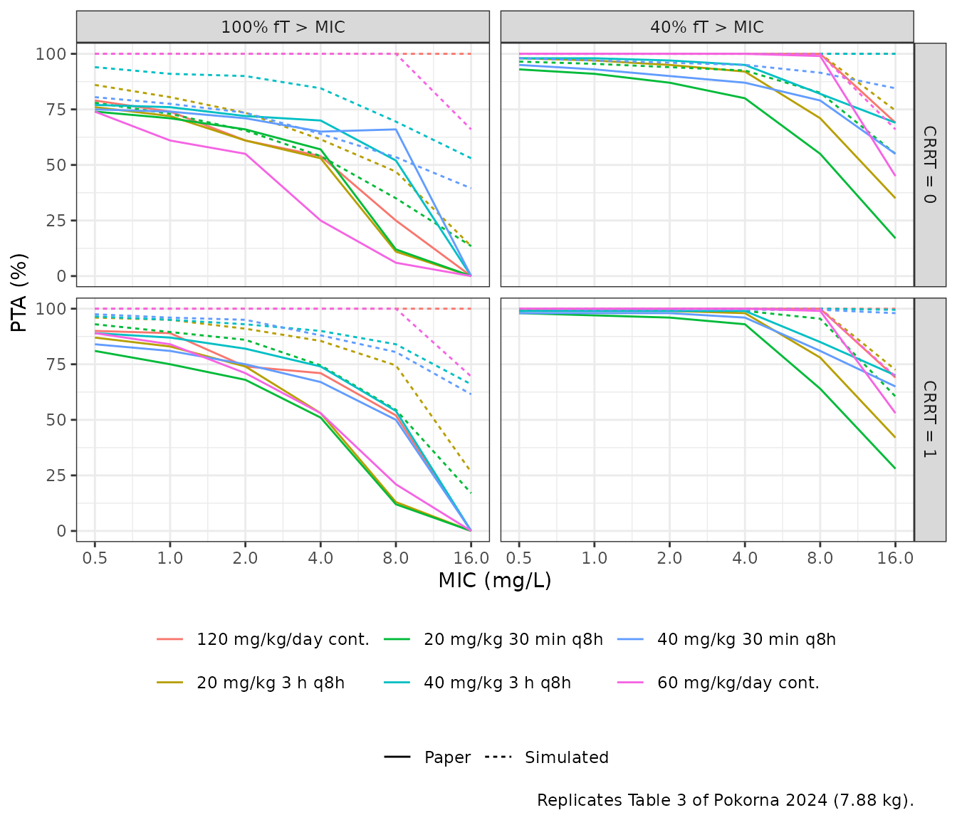
The model reproduces the shape of Table 3 but not its level. The simulated PTA is higher than the published value in 122 of the 144 cells, and the gap grows with the MIC: for 20 mg/kg over 30 min without CRRT at an MIC of 8 mg/L, 82% simulated against 55% published. The intermittent-regimen cells for 100% fT > MIC at MICs up to 4 mg/L agree more closely, with a median absolute difference of 12 points.
Table 3 cannot be reproduced from Table 2 for the continuous
infusions in particular. At steady state the concentration of a
continuous infusion is rate / CL, constant over the
interval, so the PTA for 40% and for 100% fT > MIC must be
essentially equal and must be the same on and off CRRT (V does not enter
rate / CL). Table 3 instead gives, for 60 mg/kg/day at an
MIC of 0.5 mg/L, 100% for the 40% target and 74% for the 100% target,
and different values on and off CRRT. Doubling the dose from 60 to 120
mg/kg/day moves the PTA at 16 mg/L only from 45% to 69%, which with the
Table 2 CL variability (omega^2 0.0887, a log-scale SD of 0.30) would
need a log-scale SD of about 1.1 in the steady-state concentration. The
supplementary Table S2 also lists 0% at an MIC of 16 mg/L for every
regimen for the 40% target, where Table 3 gives 17-70%. The simulation
settings behind the tables (whether residual error was added, the
evaluation window, and the protein-binding correction) are not reported,
so the published PTA values are shown for reference and are not used as
a validation target.
cell <- function(reg, crrt, tgt, mic) {
  v <- pta$Simulated[pta$regimen == reg & pta$CRRT == crrt & pta$target == tgt & pta$MIC == mic]
  if (length(v) != 1L) stop("no unique row for ", reg, " CRRT ", crrt, " target ", tgt, " MIC ", mic)
  v
}
# Model-internal properties that hold for any cohort, each far from its
# threshold relative to the binomial SE at n = 200 (at most 3.5 points):
# a continuous infusion at a low MIC attains both targets in essentially
# everyone, and 120 mg/kg/day keeps the typical steady state (36 mg/L) well
# above 16 mg/L.
stopifnot(
  cell("60 mg/kg/day cont.", 0, "100", 1) > 95,
  cell("60 mg/kg/day cont.", 1, "100", 1) > 95,
  cell("120 mg/kg/day cont.", 0, "40", 16) > 90,
  cell("20 mg/kg 30 min q8h", 0, "40", 0.5) > 85
)
Assumptions and deviations
- Scale of the IIV and residual rows. Table 2 labels the IIV rows ‘CL (%)’ and ‘Vd (%)’ but prints 0.0887 and 0.916, and the residual row ‘Proportional’ 0.17, with no control stream in the supplement. They are read here as NONMEM variances (omega^2 and sigma^2), giving a log-scale SD of 0.30 on CL and 0.96 on V and a proportional residual SD of 0.41. Read as SDs or CV fractions, CL variability would be about 9% and the residual error 17%, which cannot produce the spread of Figure 2: observed concentrations range about 5-35 mg/L at an individual prediction of 15 mg/L, and about 2-45 mg/L at a population prediction of 15 mg/L.
-
CRRT as a time-varying covariate. The Table 2
footnote defines
CRRT_onas CRRT treatment on (1) or off (0), and the Results count concentrations drawn during and off CRRT, so it is carried asRRT_CRRT_ACTIVE, the time-varying gate. The paper’s(1 + thetaCRRT)^CRRT_onis written as1 + e_crrt_vc * RRT_CRRT_ACTIVE, which is identical for a 0/1 indicator. - Covariate cohort. Body weight is drawn from a split log-normal matching the Table 1 median and IQR and truncated to 2-25 kg; 60% of subjects are on CRRT throughout, matching the fraction of concentrations drawn during CRRT. These are assumptions for illustration only.
- 25th-percentile weight. Methods 4.5 says the PTA simulations used 3.92 kg for the 25th percentile, while Table 1, the Discussion and Table S2 give 3.62 kg. Only the 7.88 kg table is replicated here.
- Table 1 units. Table 1 prints AST and ALT medians of 0.96 and 0.66 IU/L and an ECMO flow of 360 L/min, which read as other units (likely ukat/L and mL/min). These covariates were not retained and do not affect the model.
- PTA tables. Table 3 and Table S2 could not be reproduced from the Table 2 parameters (see the Table 3 section); the published values are displayed for comparison only.
- No errata were found for this article (Europe PMC, which also indexes PubMed records, checked October 2026).