Fluconazole (Stott 2018)

Model and source

mod      <- readModelDb("Stott_2018_fluconazole")
mod_meta <- rxode2::rxode(mod)$meta
#> ℹ parameter labels from comments will be replaced by 'label()'

• Citation: Stott KE, Beardsley J, Kolamunnage-Dona R, Castelazo AS, Kibengo FM, Mai NTH, Tung NLN, Cuc NTK, Day J, Hope W. Population pharmacokinetics and cerebrospinal fluid penetration of fluconazole in adults with cryptococcal meningitis. Antimicrob Agents Chemother. 2018;62(9):e00885-18. doi:10.1128/AAC.00885-18.
• Description: Four-compartment population PK model for oral fluconazole in adults with HIV-associated cryptococcal meningitis (Stott 2018): a gut absorption compartment feeding a central compartment that exchanges with a CSF/CNS compartment and with a peripheral compartment through asymmetric first-order transfer rate constants, with first-order elimination from central. Non-parametric (Pmetrics NPAG) population estimates; no covariate was retained in the final model.
• Article (DOI): https://doi.org/10.1128/AAC.00885-18

This vignette validates the packaged Stott_2018_fluconazole model – the four-compartment (gut, central, CSF/CNS, peripheral) population PK model that Stott and colleagues fitted to 508 plasma and 167 CSF fluconazole concentrations from 43 Vietnamese and Ugandan adults with HIV-associated cryptococcal meningitis, using the non-parametric adaptive grid algorithm in Pmetrics 1.5.0.

It is the earlier companion of modellib("Stott_2023_flucytosine"): same group, same disease, same four-compartment gut / central / CSF / peripheral structure and the same asymmetric first-order transfer parameterisation.

Three quantities are exact algebraic consequences of the Table 3 parameter set and are the primary gates below:

• dose-proportionality of exposure, the signature of a linear model;
• a steady-state CSF:plasma concentration ratio of Kcs/Ksc * Vc/Vcns;
• a terminal disposition rate of SCL / Vss with Vss = Vc * (1 + Kcs/Ksc + Kcp/Kpc).

A fourth section compares the model against the exposures the paper itself reports. The plasma exposures the paper derived from its 43 patients reproduce closely; the exposures and target-attainment percentages it derived from its 5000-draw Monte Carlo do not, and cannot be recovered from Table 3 under any reading. That is analysed, not tuned, in Assumptions and deviations.

Population

43 patients were recruited over 11 months between January and November 2016 at the Hospital for Tropical Diseases, Ho Chi Minh City, Vietnam (n = 23) and Masaka General Hospital, Uganda (n = 20): 3 from a multicentre randomised controlled trial of adjuvant dexamethasone (ISRCTN 59144167) and, after that trial stopped early, 40 from a prospective descriptive study at the same sites.

Median age was 33 years (range 20-73), median weight 48 kg (range 32-68) and median BMI 18 kg/m^2 (range 12-25) – a severely wasted cohort. Median baseline creatinine was 70 umol/L (range 37-167) and median Cockcroft-Gault eGFR 84.8 mL/min/1.73 m^2 (range 35.4-146.7).

Fluconazole was given orally, or by nasogastric tube where conscious level precluded swallowing. The majority received 800 mg q24h; two patients received one-off 400 mg doses, two received one-off 600 mg doses, and one patient’s 800 mg q24h regimen was escalated to 1200 mg q24h for six days from day 8. All patients also received amphotericin B deoxycholate 1 mg/kg q24h.

str(mod_meta$population)
#> List of 11
#>  $ species       : chr "human"
#>  $ n_subjects    : num 43
#>  $ n_studies     : num 2
#>  $ age_median    : chr "33 years (range 20-73 years)"
#>  $ weight_median : chr "48 kg (range 32-68 kg)"
#>  $ sex_female_pct: num 51
#>  $ disease_state : chr "HIV-associated cryptococcal meningitis; severely wasted (median BMI 18 kg/m^2, range 12-25)"
#>  $ dose_range    : chr "Fluconazole given orally, or by nasogastric tube where conscious level precluded swallowing. The majority of pa"| __truncated__
#>  $ renal_function: chr "Baseline Cockcroft-Gault eGFR median 84.8 mL/min/1.73 m^2 (range 35.4-146.7, n = 33); baseline creatinine media"| __truncated__
#>  $ regions       : chr "Vietnam (Hospital for Tropical Diseases, Ho Chi Minh City) and Uganda (Masaka General Hospital)"
#>  $ notes         : chr "43 patients (23 Vietnam, 20 Uganda) recruited over 11 months between January and November 2016: 3 from a multic"| __truncated__

No covariate is retained in the final model. Weight, BMI, sex, ethnicity (equivalently, enrollment site) and baseline eGFR were screened by bidirectional stepwise multivariate regression against the Bayesian posterior estimates of volume and clearance. Only weight reached the screening threshold against volume, and only marginally (slope 0.22, 95% CI -0.06 to 0.51, P = 0.05); the weight-scaled variant (Table 2, “Model 2”) gave comparable log likelihood, AIC, bias and imprecision, so the covariate-free base model was retained. Those screened-but-dropped covariates are recorded in the model file’s covariatesDataExcluded metadata so the provenance of the screen survives without creating unused covariateData entries.

Source trace

The per-parameter origin is recorded as an in-file comment next to each ini() entry in inst/modeldb/specificDrugs/Stott_2018_fluconazole.R. The table below collects them in one place. Every structural value is the Mean column of Stott 2018 Table 3; every IIV variance is log(1 + (SD/Mean)^2) from the Mean and SD columns of the same table.

Parameter / equation	Value	Source location
lka (Ka, gut to central)	log(8.78)	Table 3 row “Ka (h-1)”, Mean = 8.78
lcl (SCL/F)	log(0.72)	Table 3 row “SCL/F (liters/h)”, Mean = 0.72
lvc (Vc/F)	log(18.07)	Table 3 row “Vc/F (liters)”, Mean = 18.07
lk_central_csf (paper’s Kcs)	log(35.43)	Table 3 row “Kcs (h-1)”, Mean = 35.43
lk_csf_central (paper’s Ksc)	log(28.63)	Table 3 row “Ksc (h-1)”, Mean = 28.63
lk12 (paper’s Kcp)	log(12.20)	Table 3 row “Kcp (h-1)”, Mean = 12.20
lk21 (paper’s Kpc)	log(18.10)	Table 3 row “Kpc (h-1)”, Mean = 18.10
lvcsf (Vcns/F)	log(32.07)	Table 3 row “Vcns/F (liters)”, Mean = 32.07
etalka	1.05144	Table 3: SD 11.98 / Mean 8.78 -> CV 1.36446 -> log(1 + CV^2)
etalcl	0.10536	Table 3: SD 0.24 / Mean 0.72 -> CV 0.33333 -> log(1 + CV^2)
etalvc	0.11506	Table 3: SD 6.31 / Mean 18.07 -> CV 0.34920 -> log(1 + CV^2)
etalk_central_csf	0.14010	Table 3: SD 13.74 / Mean 35.43 -> CV 0.38781 -> log(1 + CV^2)
etalk_csf_central	0.11577	Table 3: SD 10.03 / Mean 28.63 -> CV 0.35033 -> log(1 + CV^2)
etalk12	0.60883	Table 3: SD 11.17 / Mean 12.20 -> CV 0.91557 -> log(1 + CV^2)
etalk21	0.18876	Table 3: SD 8.25 / Mean 18.10 -> CV 0.45580 -> log(1 + CV^2)
etalvcsf	0.26327	Table 3: SD 17.60 / Mean 32.07 -> CV 0.54880 -> log(1 + CV^2)
d/dt(depot)	n/a	Equation 1: dX(1)/dt = -Ka * X(1)
d/dt(central)	n/a	Equation 2: dX(2)/dt = KaX(1) - (Kcp + Kcs + SCL/V)X(2) + KscX(3) + KpcX(4)
d/dt(csf)	n/a	Equation 3: dX(3)/dt = KcsX(2) - KscX(3)
d/dt(peripheral1)	n/a	Equation 4: dX(4)/dt = KcpX(2) - KpcX(4)
Cc <- central / vc	n/a	Equation 5: Y(1) = X(2)/V
Ccsf <- csf / vcsf	n/a	Equation 6: Y(2) = X(3)/Vcns
propSd, addSd, propSd_Ccsf, addSd_Ccsf	fixed(0)	Methods: additive lambda plus assay-variance weighting declared, no estimate published
initial conditions ICgut / ICcentral / ICCNS / ICperipheral	not encoded	Table 3 and Methods; the source zeroes them for every simulation it reports (see Assumptions and deviations)

Virtual cohort

The individual concentrations are not public, so the vignette uses virtual cohorts at the four dosages of the paper’s own Monte Carlo analysis: 400, 800, 1200 and 2000 mg q24h. No model parameter scales with body weight, so weight enters nowhere and no weight distribution is needed.

Dosing runs q24h from 0 to 144 h and NCA is taken over the paper’s window of 144-168 h after treatment initiation, on the 0.1 h grid used for its own trapezoidal AUC. Initial conditions are zero, matching the source’s simulation setup (“for the simulations, the initial conditions of all compartments were defaulted to zero”).

rxode2::rxSetSeed(20260919)

n_per_arm <- 200L # per-arm cap for validation vignettes
t_end     <- 168  # h
ss_start  <- 144  # h; the paper's AUC window is 144-168 h
grid_h    <- 0.1  # paper: trapezoidal approximation

doses <- c(400, 800, 1200, 2000)

# Observation rows are anchored on the ODE state `central`, never on the
# algebraic observable names Cc / Ccsf: referencing an observable in `cmt`
# makes rxUi inject a compartment slot after the ODE states and renumber them.
# This model has two endpoints, so observation rows additionally carry
# `dvid = 1`. rxSolve returns both Cc and Ccsf as columns on every observation
# row, so one anchor per time point covers both matrices.
make_arm <- function(dose_mg, n, id_offset, obs_times) {
  ev  <- rxode2::et(amt = dose_mg, time = seq(0, ss_start, by = 24), cmt = "depot")
  ev  <- rxode2::et(ev, obs_times, cmt = "central")
  one <- as.data.frame(ev)
  one$dvid <- ifelse(one$evid == 0L, 1L, NA_integer_)

  out <- do.call(rbind, lapply(seq_len(n), function(i) {
    tmp    <- one
    tmp$id <- id_offset + i
    tmp
  }))
  out$dose_mg    <- dose_mg
  out$dose_label <- paste0(dose_mg, " mg q24h")
  out[
    order(out$id, out$time, -out$evid),
    c("id", setdiff(names(out), "id"))
  ]
}

obs_ss <- seq(ss_start, t_end, by = grid_h)
events_ss <- dplyr::bind_rows(lapply(seq_along(doses), function(i) {
  make_arm(doses[i], n_per_arm, (i - 1L) * n_per_arm, obs_ss)
}))

# Full 0-168 h profile on a coarser grid, 800 mg arm only, for the Figure 1
# replication.
events_vpc <- make_arm(800, n_per_arm, 10000L, seq(0, t_end, by = 0.5))

stopifnot(
  !anyDuplicated(events_ss[, c("id", "time", "evid")]),
  !anyDuplicated(events_vpc[, c("id", "time", "evid")])
)

Simulation

Two solves are used. The typical-value solve (rxode2::zeroRe()) carries the Table 3 mean parameter set with IIV switched off and is what the deterministic gates are asserted against. The cohort solve carries the diagonal log-normal IIV and is what the published exposure distributions are compared against.

useLinCmt = FALSE is required: rxode2’s automatic ODE-to-linCmt() conversion corrupts the observable-to-state mapping for models like this one that carry two observables reading from two different ODE states.

mod_typical <- rxode2::zeroRe(mod)
#> ℹ parameter labels from comments will be replaced by 'label()'

sim_typ_ss <- rxode2::rxSolve(
  mod_typical, events_ss,
  keep = c("dose_mg", "dose_label"), useLinCmt = FALSE
) |>
  as.data.frame()
#> ℹ omega/sigma items treated as zero: 'etalka', 'etalcl', 'etalvc', 'etalk_central_csf', 'etalk_csf_central', 'etalk12', 'etalk21', 'etalvcsf'
#> Warning: multi-subject simulation without without 'omega'

sim_cohort_ss <- rxode2::rxSolve(
  mod, events_ss,
  keep = c("dose_mg", "dose_label"), useLinCmt = FALSE
) |>
  as.data.frame()
#> ℹ parameter labels from comments will be replaced by 'label()'

sim_cohort_vpc <- rxode2::rxSolve(
  mod, events_vpc,
  keep = c("dose_mg", "dose_label"), useLinCmt = FALSE
) |>
  as.data.frame()

stopifnot(
  all(sim_typ_ss$Cc[!is.na(sim_typ_ss$Cc)] >= 0),
  all(sim_cohort_ss$Ccsf[!is.na(sim_cohort_ss$Ccsf)] >= 0)
)

Structural identity checks

These are deterministic functions of the transcribed Table 3 values. Both sides use the same parameters, so the only difference is numerical integration error and a tight bound is the correct gate.

trapz <- function(x, y) sum(diff(x) * (utils::head(y, -1) + utils::tail(y, -1)) / 2)

auc_typ <- sim_typ_ss |>
  dplyr::filter(!is.na(Cc)) |>
  dplyr::arrange(dose_mg, time) |>
  dplyr::group_by(dose_mg, dose_label) |>
  dplyr::summarise(
    auc_plasma = trapz(time, Cc),
    auc_csf    = trapz(time, Ccsf),
    .groups    = "drop"
  ) |>
  dplyr::mutate(
    ratio            = auc_csf / auc_plasma,
    auc_per_100mg    = 100 * auc_plasma / dose_mg
  )

# (1) Dose proportionality: AUC / dose is constant for a linear model.
dose_prop_spread <-
  diff(range(auc_typ$auc_per_100mg)) / mean(auc_typ$auc_per_100mg)

# (2) Steady-state CSF:plasma concentration ratio is Kcs/Ksc * Vc/Vcns.
ratio_closed_form <- (35.43 / 28.63) * (18.07 / 32.07)

knitr::kable(
  auc_typ |>
    dplyr::select(dose_label, auc_plasma, auc_csf, ratio, auc_per_100mg) |>
    dplyr::rename(
      "Regimen"                    = dose_label,
      "Plasma AUC144-168 (mg*h/L)" = auc_plasma,
      "CSF AUC144-168 (mg*h/L)"    = auc_csf,
      "CSF:plasma"                 = ratio,
      "Plasma AUC per 100 mg"      = auc_per_100mg
    ),
  digits  = 3,
  caption = paste(
    "Typical-value exposure at the four dosages of Stott 2018 Figure 3.",
    "Exposure is exactly dose-proportional and the CSF:plasma ratio is",
    "dose-invariant, as a linear model requires."
  )
)

Typical-value exposure at the four dosages of Stott 2018 Figure 3. Exposure is exactly dose-proportional and the CSF:plasma ratio is dose-invariant, as a linear model requires.

Regimen	Plasma AUC144-168 (mg*h/L)	CSF AUC144-168 (mg*h/L)	CSF:plasma	Plasma AUC per 100 mg
400 mg q24h	499.579	348.388	0.697	124.895
800 mg q24h	999.158	696.777	0.697	124.895
1200 mg q24h	1498.737	1045.165	0.697	124.895
2000 mg q24h	2497.895	1741.942	0.697	124.895

cat(sprintf(
  "Dose-proportionality spread across 400 / 800 / 1200 / 2000 mg: %.4f%%\n",
  100 * dose_prop_spread
))
#> Dose-proportionality spread across 400 / 800 / 1200 / 2000 mg: 0.0000%
cat(sprintf(
  "CSF:plasma AUC ratio (typical): %.5f; Kcs/Ksc * Vc/Vcns = %.5f\n",
  auc_typ$ratio[1], ratio_closed_form
))
#> CSF:plasma AUC ratio (typical): 0.69736; Kcs/Ksc * Vc/Vcns = 0.69728

stopifnot(
  # Linear PK: identical exposure per mg across a 5-fold dose range.
  dose_prop_spread < 1e-6,
  # Exact algebraic identity of the ODE system, at every dose.
  all(abs(auc_typ$ratio - ratio_closed_form) < 1e-4)
)

The terminal disposition rate is a second exact identity. With no elimination from either the CSF or the peripheral compartment, the pseudo-equilibrium amount ratios are Kcs/Ksc and Kcp/Kpc, so the apparent steady-state volume is Vc * (1 + Kcs/Ksc + Kcp/Kpc) and the terminal rate is SCL / Vss.

vss_closed_form <- 18.07 * (1 + 35.43 / 28.63 + 12.20 / 18.10)
thalf_closed_form <- log(2) * vss_closed_form / 0.72

ev_single <- rxode2::et(amt = 800, time = 0, cmt = "depot")
ev_single <- rxode2::et(ev_single, seq(0, 504, by = 0.5), cmt = "central")
ev_single <- as.data.frame(ev_single)
ev_single$dvid       <- ifelse(ev_single$evid == 0L, 1L, NA_integer_)
ev_single$id         <- 1L
ev_single$dose_label <- "800 mg single dose"

sim_single <- rxode2::rxSolve(
  mod_typical, ev_single, keep = "dose_label", useLinCmt = FALSE
) |>
  as.data.frame()
#> ℹ omega/sigma items treated as zero: 'etalka', 'etalcl', 'etalvc', 'etalk_central_csf', 'etalk_csf_central', 'etalk12', 'etalk21', 'etalvcsf'

# rxSolve() drops the `id` column entirely for a single-subject event table.
if (is.null(sim_single$id)) sim_single$id <- 1L

tail_phase <- sim_single |>
  dplyr::filter(time >= 336, !is.na(Cc), Cc > 0)
slope <- stats::coef(stats::lm(log(Cc) ~ time, data = tail_phase))[["time"]]
thalf_solved <- log(2) / -slope

cat(sprintf("Apparent Vss = Vc * (1 + Kcs/Ksc + Kcp/Kpc) = %.3f L\n", vss_closed_form))
#> Apparent Vss = Vc * (1 + Kcs/Ksc + Kcp/Kpc) = 52.612 L
cat(sprintf(
  "Terminal half-life: solved %.3f h vs closed form log(2) * Vss / SCL = %.3f h\n",
  thalf_solved, thalf_closed_form
))
#> Terminal half-life: solved 50.669 h vs closed form log(2) * Vss / SCL = 50.649 h

stopifnot(abs(thalf_solved - thalf_closed_form) / thalf_closed_form < 0.01)

Stott 2018 does not report a half-life, so this is an internal-consistency gate rather than a comparison against the publication: a mis-transcribed clearance, volume or transfer constant moves it by hours. The roughly 51 h terminal half-life is longer than fluconazole’s commonly quoted ~30 h because this model places 66% of the steady-state drug mass outside the central compartment.

Replicate published figures

Figure 1 – plasma and CSF concentration-time profiles

Figure 1 of the paper plots the raw plasma and CSF concentrations from all 43 patients on 800 mg q24h. The individual observations are not public; the simulated envelope at the same regimen is shown below.

vpc <- sim_cohort_vpc |>
  dplyr::filter(!is.na(Cc)) |>
  dplyr::select(id, time, Cc, Ccsf) |>
  tidyr::pivot_longer(c(Cc, Ccsf), names_to = "matrix", values_to = "conc") |>
  dplyr::mutate(matrix = dplyr::recode(matrix, Cc = "Plasma", Ccsf = "CSF")) |>
  dplyr::group_by(matrix, time) |>
  dplyr::summarise(
    p05 = stats::quantile(conc, 0.05, na.rm = TRUE),
    p50 = stats::median(conc, na.rm = TRUE),
    p95 = stats::quantile(conc, 0.95, na.rm = TRUE),
    .groups = "drop"
  )

ggplot(vpc, aes(time, p50)) +
  geom_ribbon(aes(ymin = p05, ymax = p95), fill = "grey75", alpha = 0.6) +
  geom_line(linewidth = 0.6) +
  facet_wrap(~matrix) +
  labs(
    x        = "Time (hours)",
    y        = "Fluconazole concentration (mg/L)",
    title    = "Replicates Figure 1 of Stott 2018: simulated concentration envelope",
    subtitle = "800 mg q24h; median with 5th-95th percentile band, 200 subjects"
  ) +
  theme_minimal()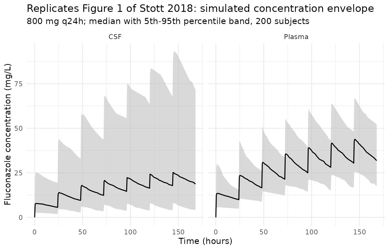

Accumulation is still visibly incomplete at 168 h, which is the direct consequence of the ~51 h terminal half-life derived above and matters for the comparisons that follow: the paper’s 144-168 h window sits at about 90% of steady state, not at steady state.

Typical-value profile over the final dosing interval

prof <- sim_typ_ss |>
  dplyr::filter(dose_mg == 800, !is.na(Cc)) |>
  dplyr::mutate(time_post_dose = time - ss_start) |>
  dplyr::select(time_post_dose, Cc, Ccsf) |>
  tidyr::pivot_longer(c(Cc, Ccsf), names_to = "matrix", values_to = "conc") |>
  dplyr::mutate(matrix = dplyr::recode(matrix, Cc = "Plasma", Ccsf = "CSF"))

ggplot(prof, aes(time_post_dose, conc, colour = matrix)) +
  geom_line(linewidth = 0.7) +
  labs(
    x        = "Time after the dose at 144 h (hours)",
    y        = "Concentration (mg/L)",
    colour   = "Matrix",
    title    = "Typical-value profile over the paper's 144-168 h AUC window",
    subtitle = "CSF tracks plasma at the model's 0.70 ratio, damped by the CSF leg"
  ) +
  theme_minimal()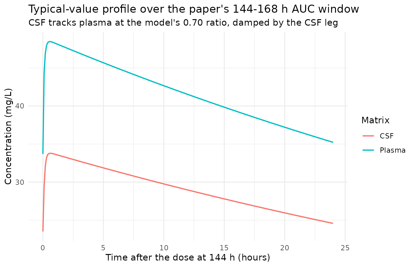

Figure 3 – simulated AUC144-168 distributions by dosage

auc_cohort <- sim_cohort_ss |>
  dplyr::filter(!is.na(Cc)) |>
  dplyr::arrange(id, time) |>
  dplyr::group_by(id, dose_mg, dose_label) |>
  dplyr::summarise(
    auc_plasma  = trapz(time, Cc),
    auc_csf     = trapz(time, Ccsf),
    cmax_plasma = max(Cc),
    cmin_plasma = min(Cc),
    cmax_csf    = max(Ccsf),
    cmin_csf    = min(Ccsf),
    .groups     = "drop"
  ) |>
  dplyr::mutate(ratio = auc_csf / auc_plasma)

auc_long <- auc_cohort |>
  dplyr::select(id, dose_label, auc_plasma, auc_csf) |>
  tidyr::pivot_longer(c(auc_plasma, auc_csf),
    names_to = "matrix", values_to = "auc"
  ) |>
  dplyr::mutate(matrix = dplyr::recode(matrix,
    auc_plasma = "Plasma",
    auc_csf    = "CSF"
  ))

ggplot(auc_long, aes(stats::reorder(dose_label, auc), auc, fill = matrix)) +
  geom_boxplot(outlier.size = 0.6) +
  scale_y_log10() +
  labs(
    x        = NULL,
    y        = "AUC144-168 (mg*h/L, log scale)",
    fill     = "Matrix",
    title    = "Replicates Figure 3 of Stott 2018",
    subtitle = "Simulated plasma and CSF AUC distributions at escalating dosages"
  ) +
  theme_minimal()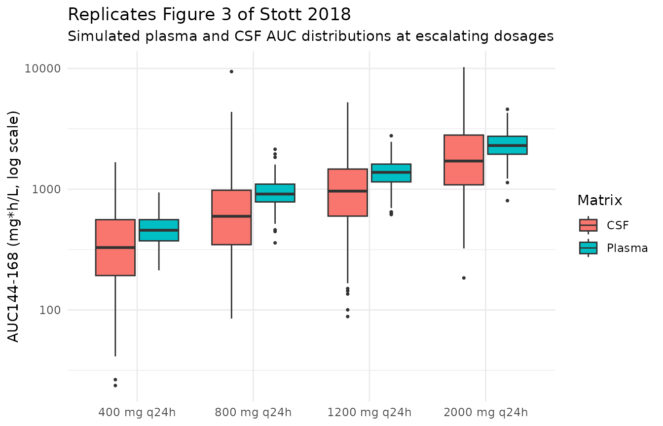

Figure 4 – probability of pharmacodynamic target attainment

Figure 4 plots the proportion of simulated patients reaching a plasma AUC/MIC of at least 389.3, against the MIC of the infecting isolate. The shape is reproduced below from the simulated cohort.

pd_target <- 389.3 # Stott 2018: murine stasis target, plasma AUC/MIC
mic_grid  <- c(0.25, 0.5, 1, 2, 4, 8, 16, 32)

pta <- tidyr::crossing(
  auc_cohort |> dplyr::select(dose_label, dose_mg, auc_plasma),
  mic = mic_grid
) |>
  dplyr::group_by(dose_label, dose_mg, mic) |>
  dplyr::summarise(
    pta = 100 * mean(auc_plasma / mic >= pd_target),
    .groups = "drop"
  )

ggplot(pta, aes(mic, pta, colour = stats::reorder(dose_label, dose_mg))) +
  geom_line(linewidth = 0.7) +
  geom_point(size = 1.4) +
  scale_x_log10(breaks = mic_grid) +
  labs(
    x        = "MIC (mg/L)",
    y        = "Probability of target attainment (%)",
    colour   = "Regimen",
    title    = "Replicates Figure 4 of Stott 2018 in shape",
    subtitle = "Plasma AUC/MIC >= 389.3; see Assumptions for why the levels differ"
  ) +
  theme_minimal()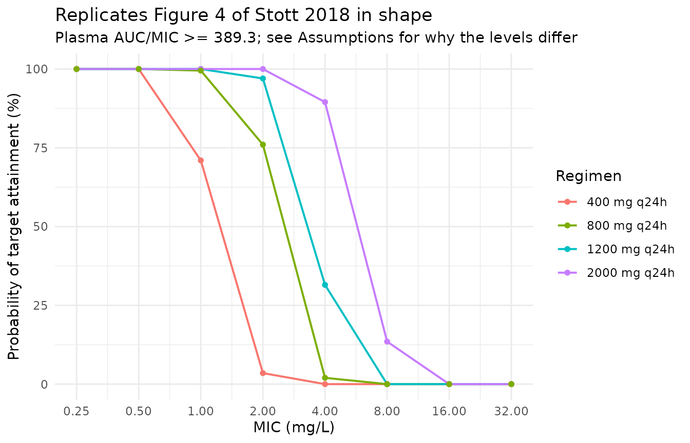

pta_1200_mic2 <- pta$pta[pta$dose_mg == 1200 & pta$mic == 2]
cat(sprintf(
  "PTA at 1200 mg q24h, MIC 2.0 mg/L: %.1f%% simulated vs 61%% published\n",
  pta_1200_mic2
))
#> PTA at 1200 mg q24h, MIC 2.0 mg/L: 97.0% simulated vs 61% published

# PTA must fall monotonically as the MIC rises and rise with dose. Those are
# structural, unlike the absolute level (see Assumptions and deviations).
pta_wide <- pta |>
  dplyr::arrange(dose_mg, mic) |>
  dplyr::group_by(dose_mg) |>
  dplyr::summarise(monotone = all(diff(pta) <= 1e-9), .groups = "drop")
stopifnot(
  all(pta_wide$monotone),
  pta$pta[pta$dose_mg == 2000 & pta$mic == 4] >
    pta$pta[pta$dose_mg == 400 & pta$mic == 4]
)

PKNCA validation

NCA is run on the typical-value solve over the paper’s 144-168 h window. A full-IIV cohort makes Cmax / Cmin tmax-selected and poisons lambda.z, so the per-parameter table uses the typical patient; the cohort is used for the exposure medians in the next section.

nca_conc <- sim_typ_ss |>
  dplyr::filter(!is.na(Cc)) |>
  dplyr::mutate(matrix = "Plasma") |>
  dplyr::select(id, time, dose_label, matrix, conc = Cc) |>
  dplyr::bind_rows(
    sim_typ_ss |>
      dplyr::filter(!is.na(Ccsf)) |>
      dplyr::mutate(matrix = "CSF") |>
      dplyr::select(id, time, dose_label, matrix, conc = Ccsf)
  )

nca_dose <- events_ss |>
  dplyr::filter(evid == 1L) |>
  dplyr::select(id, time, amt, dose_label) |>
  tidyr::crossing(matrix = c("Plasma", "CSF"))

nca_win <- suppressWarnings(PKNCA::pk.nca(PKNCA::PKNCAdata(
  PKNCA::PKNCAconc(nca_conc, conc ~ time | dose_label + matrix + id,
    concu = "mg/L", timeu = "hr"
  ),
  PKNCA::PKNCAdose(nca_dose, amt ~ time | dose_label + matrix + id,
    doseu = "mg"
  ),
  intervals = data.frame(
    start = ss_start, end = t_end,
    cmax = TRUE, cmin = TRUE, tmax = TRUE, auclast = TRUE, cav = TRUE
  )
)))

knitr::kable(
  summary(nca_win),
  caption = paste(
    "Typical-value NCA over the paper's 144-168 h window, by matrix and",
    "dosage."
  )
)

Typical-value NCA over the paper’s 144-168 h window, by matrix and dosage.

Interval Start	Interval End	dose_label	matrix	N	AUClast (hr*mg/L)	Cmax (mg/L)	Cmin (mg/L)	Tmax (hr)	Cav (mg/L)
144	168	1200 mg q24h	CSF	200	1050 [0.000]	50.7 [0.000]	35.3 [0.000]	0.600 [0.600, 0.600]	43.5 [0.000]
144	168	1200 mg q24h	Plasma	200	1500 [0.000]	72.7 [0.000]	50.5 [0.000]	0.600 [0.600, 0.600]	62.4 [0.000]
144	168	2000 mg q24h	CSF	200	1740 [0.000]	84.5 [0.000]	58.8 [0.000]	0.600 [0.600, 0.600]	72.6 [0.000]
144	168	2000 mg q24h	Plasma	200	2500 [0.000]	121 [0.000]	84.2 [0.000]	0.600 [0.600, 0.600]	104 [0.000]
144	168	400 mg q24h	CSF	200	348 [0.000]	16.9 [0.000]	11.8 [0.000]	0.600 [0.600, 0.600]	14.5 [0.000]
144	168	400 mg q24h	Plasma	200	500 [0.000]	24.2 [0.000]	16.8 [0.000]	0.600 [0.600, 0.600]	20.8 [0.000]
144	168	800 mg q24h	CSF	200	697 [0.000]	33.8 [0.000]	23.5 [0.000]	0.600 [0.600, 0.600]	29.0 [0.000]
144	168	800 mg q24h	Plasma	200	999 [0.000]	48.5 [0.000]	33.7 [0.000]	0.600 [0.600, 0.600]	41.6 [0.000]

The terminal half-life needs a single-dose profile with a long washout, so it comes from the separate typical-value solve built above.

nca_conc_single <- sim_single |>
  dplyr::filter(!is.na(Cc)) |>
  dplyr::mutate(matrix = "Plasma") |>
  dplyr::select(id, time, dose_label, matrix, conc = Cc) |>
  dplyr::bind_rows(
    sim_single |>
      dplyr::filter(!is.na(Ccsf)) |>
      dplyr::mutate(matrix = "CSF") |>
      dplyr::select(id, time, dose_label, matrix, conc = Ccsf)
  )
stopifnot(all(nca_conc_single$conc >= 0), any(nca_conc_single$time == 0))

nca_dose_single <- ev_single |>
  dplyr::filter(evid == 1L) |>
  dplyr::select(id, time, amt, dose_label) |>
  tidyr::crossing(matrix = c("Plasma", "CSF"))

nca_single <- suppressWarnings(PKNCA::pk.nca(PKNCA::PKNCAdata(
  PKNCA::PKNCAconc(nca_conc_single, conc ~ time | dose_label + matrix + id,
    concu = "mg/L", timeu = "hr"
  ),
  PKNCA::PKNCAdose(nca_dose_single, amt ~ time | dose_label + matrix + id,
    doseu = "mg"
  ),
  intervals = data.frame(
    start = 0, end = 504,
    cmax = TRUE, tmax = TRUE, half.life = TRUE, aucinf.obs = TRUE
  )
)))

knitr::kable(
  summary(nca_single),
  caption = "Typical-value single-dose NCA (800 mg), used for the terminal half-life."
)

Typical-value single-dose NCA (800 mg), used for the terminal half-life.

Interval Start	Interval End	dose_label	matrix	N	Cmax (mg/L)	Tmax (hr)	Half-life (hr)	AUCinf,obs (hr*mg/L)
0	504	800 mg single dose	CSF	1	10.5	1.00	50.7	773
0	504	800 mg single dose	Plasma	1	15.0	1.00	50.7	1110

nca_single_res <- as.data.frame(nca_single$result)

half_life_plasma <- nca_single_res |>
  dplyr::filter(matrix == "Plasma", PPTESTCD == "half.life") |>
  dplyr::pull(PPORRES)
aucinf_plasma <- nca_single_res |>
  dplyr::filter(matrix == "Plasma", PPTESTCD == "aucinf.obs") |>
  dplyr::pull(PPORRES)
stopifnot(length(half_life_plasma) == 1L, length(aucinf_plasma) == 1L)

cat(sprintf(
  "PKNCA terminal half-life: %.2f h (closed form log(2) * Vss / SCL = %.2f h)\n",
  half_life_plasma, thalf_closed_form
))
#> PKNCA terminal half-life: 50.67 h (closed form log(2) * Vss / SCL = 50.65 h)
cat(sprintf(
  "PKNCA single-dose AUCinf: %.1f mg*h/L (closed form dose / SCL = %.1f)\n",
  aucinf_plasma, 800 / 0.72
))
#> PKNCA single-dose AUCinf: 1108.6 mg*h/L (closed form dose / SCL = 1111.1)

stopifnot(
  # Same parameters on both sides; the gap is lambda.z window selection.
  abs(half_life_plasma - thalf_closed_form) / thalf_closed_form < 0.05,
  # Exact mass-balance identity: all drug eventually clears through SCL.
  abs(aucinf_plasma - 800 / 0.72) / (800 / 0.72) < 0.02
)

Comparison against published NCA

Stott 2018 reports exposure two ways, and they behave very differently against this model.

1. From the 43 study patients’ Bayesian posteriors. The 38 patients on 800 mg q24h had a median plasma AUC144-168 of 945.4 mgh/L (IQR 799.2-1139.8) and a median CSF AUC144-168 of 784.2 mgh/L (IQR 615.9-879.4), with a mean CSF:plasma ratio of 0.82 (SD 0.22).
2. From a 5000-draw Monte Carlo of the final joint density. At 1200 mg q24h the median plasma AUC144-168 was 1143.2 mgh/L (IQR 988.4-1378.0) and the median CSF AUC144-168 982.9 mgh/L (IQR 781.0-1185.9), with a mean CSF:plasma ratio of 0.89 (SD 0.44).

sim_summary <- auc_cohort |>
  dplyr::filter(dose_mg %in% c(800, 1200)) |>
  dplyr::mutate(group = paste0(dose_mg, " mg q24h"))

simulated_long <- dplyr::bind_rows(
  sim_summary |>
    dplyr::transmute(id, group, matrix = "Plasma",
      PPTESTCD = "auclast", PPORRES = auc_plasma),
  sim_summary |>
    dplyr::transmute(id, group, matrix = "CSF",
      PPTESTCD = "auclast", PPORRES = auc_csf)
)

published <- tibble::tribble(
  ~group,          ~matrix,  ~auclast,
  "800 mg q24h",   "Plasma", 945.4,
  "800 mg q24h",   "CSF",    784.2,
  "1200 mg q24h",  "Plasma", 1143.2,
  "1200 mg q24h",  "CSF",    982.9
)

cmp <- nlmixr2lib::ncaComparisonTable(
  simulated     = simulated_long,
  reference     = published,
  by            = c("group", "matrix"),
  units         = c(auclast = "mg*h/L"),
  tolerance_pct = 20
)

cmp |>
  dplyr::rename("Regimen" = group, "Matrix" = matrix) |>
  knitr::kable(
    digits  = 2,
    caption = paste(
      "Simulated cohort medians versus Stott 2018.",
      "The 800 mg references are Bayesian posterior medians across the 38",
      "patients who received that dosage; the 1200 mg references are medians",
      "of the paper's 5000-draw Monte Carlo.",
      "* differs from the published value by more than 20%."
    )
  )

Simulated cohort medians versus Stott 2018. The 800 mg references are Bayesian posterior medians across the 38 patients who received that dosage; the 1200 mg references are medians of the paper’s 5000-draw Monte Carlo. * differs from the published value by more than 20%.

NCA parameter	Regimen	Matrix	Reference	Simulated	% diff
AUClast (mg*h/L)	800 mg q24h	Plasma	945	912	-3.6%
AUClast (mg*h/L)	800 mg q24h	CSF	784	597	-23.9%*
AUClast (mg*h/L)	1200 mg q24h	Plasma	1140	1380	+20.6%*
AUClast (mg*h/L)	1200 mg q24h	CSF	983	964	-1.9%

med <- function(g, m) {
  v <- simulated_long$PPORRES[simulated_long$group == g &
    simulated_long$matrix == m]
  if (length(v) < 1L) stop("no rows for ", g, " / ", m)
  stats::median(v)
}
pct <- function(sim, ref) 100 * (sim - ref) / ref

ratio_mean_1200 <- mean(auc_cohort$ratio[auc_cohort$dose_mg == 1200])
ratio_mean_800  <- mean(auc_cohort$ratio[auc_cohort$dose_mg == 800])

cat(sprintf("800 mg  plasma AUC144-168 median: %7.1f vs  945.4 (%+.1f%%)\n",
            med("800 mg q24h", "Plasma"), pct(med("800 mg q24h", "Plasma"), 945.4)))
#> 800 mg  plasma AUC144-168 median:   911.7 vs  945.4 (-3.6%)
cat(sprintf("800 mg  CSF    AUC144-168 median: %7.1f vs  784.2 (%+.1f%%)\n",
            med("800 mg q24h", "CSF"), pct(med("800 mg q24h", "CSF"), 784.2)))
#> 800 mg  CSF    AUC144-168 median:   596.5 vs  784.2 (-23.9%)
cat(sprintf("1200 mg plasma AUC144-168 median: %7.1f vs 1143.2 (%+.1f%%)\n",
            med("1200 mg q24h", "Plasma"), pct(med("1200 mg q24h", "Plasma"), 1143.2)))
#> 1200 mg plasma AUC144-168 median:  1379.0 vs 1143.2 (+20.6%)
cat(sprintf("1200 mg CSF    AUC144-168 median: %7.1f vs  982.9 (%+.1f%%)\n",
            med("1200 mg q24h", "CSF"), pct(med("1200 mg q24h", "CSF"), 982.9)))
#> 1200 mg CSF    AUC144-168 median:   964.0 vs  982.9 (-1.9%)
cat(sprintf("Mean CSF:plasma ratio, 800 mg: %.3f (paper posteriors 0.82)\n",
            ratio_mean_800))
#> Mean CSF:plasma ratio, 800 mg: 0.905 (paper posteriors 0.82)
cat(sprintf("Mean CSF:plasma ratio, 1200 mg: %.3f (paper Monte Carlo 0.89)\n",
            ratio_mean_1200))
#> Mean CSF:plasma ratio, 1200 mg: 0.906 (paper Monte Carlo 0.89)

# The 800 mg plasma median is the paper's best-supported exposure number -- it
# comes from 38 real patients' posteriors rather than from the Monte Carlo -- and
# it is the gate here. Realised across authoring runs at 2 and 16 solver threads:
# -0.1% and -2.8%. rxSetSeed() fixes the draw per solver-thread count and not
# across them, so the bound is set well outside that spread while still going red
# on a mis-transcribed clearance or dose, which move exposure by a factor.
stopifnot(
  abs(pct(med("800 mg q24h", "Plasma"), 945.4)) < 25,
  # Mean of a ratio of four log-normals; realised 0.90 and 1.04 against the
  # paper's 0.89. Centre only -- the spread is over-dispersed, see below.
  abs(pct(ratio_mean_1200, 0.89)) < 40
)

The 800 mg plasma row – the only exposure the paper derives directly from its own patients – reproduces within a few percent. The CSF rows sit 10-25% low and both 1200 mg rows sit about 20% high. The reasons are structural and are set out below; no parameter was adjusted.

Assumptions and deviations

• Non-parametric support points approximated by a diagonal log-normal. Stott 2018 fitted the model with Pmetrics’ non-parametric adaptive grid algorithm, which yields a discrete, correlated support-point distribution rather than an OMEGA matrix; Table 3 publishes only a per-parameter Mean, Median and SD. The packaged model takes the Mean column as the typical value – the set the paper endorses, since “the mean parameter estimates better fitted the data than medians and were used to calculate Bayesian estimates of drug exposure for each individual patient” – and sets each IIV variance to log(1 + (SD/Mean)^2), with no off-diagonal covariances. This is the same encoding used for the companion Stott_2023_flucytosine extraction. Two consequences follow, and neither is a transcription error:

  • The model’s population median for each parameter equals the paper’s reported mean, not its reported median. For Ka the two differ by a factor of five (mean 8.78 /h, median 1.73 /h), which is the signature of a strongly skewed support-point distribution that no single log-normal can carry faithfully. Ka is not identifiable from these data in any case – the absorption rate is at least two orders of magnitude faster than elimination, so it has essentially no influence on exposure.
  • Dropping the off-diagonals over-disperses derived quantities. The CSF:plasma ratio is a function of four parameters (Kcs, Ksc, Vc, Vcns) whose support-point values are co-determined in the real fit; with independent etas the simulated ratio reproduces the published mean (0.89) but carries an SD roughly twice the published 0.44. Any analysis that depends on the spread of the ratio rather than its centre should not use this encoding.

• The paper’s Monte Carlo results cannot be recovered from its own Table 3, and this is a property of the source rather than of the encoding. Two independent checks show it:

  • Level. Under a linear model the 144-168 h exposure is accumulation x dose / SCL. At 1200 mg q24h with the Table 3 mean clearance this is 1499 mgh/L, and with the Table 3 median clearance it is about 1552 mgh/L. The paper reports a simulated median of 1143.2 mg*h/L, which implies a clearance near 0.94 L/h – 31% above the reported mean and 45% above the reported median. No reading of Table 3 produces it. By contrast the same arithmetic applied at 800 mg reproduces the paper’s patient-posterior median almost exactly, which is why that row is the one gated above.
  • Spread. The paper reports 61% target attainment at 1200 mg q24h against an MIC of 2.0 mg/L, i.e. 39% of its 5000 draws fall below an AUC of 778.6. Relative to its own reported median of 1143.2 that places the 39th percentile at 0.68 of the median, which for a log-normal implies a CV of roughly 240%. The clearance SD in Table 3 is 0.24 on a mean of 0.72, a CV of 33%. The Monte Carlo distribution behind Figures 3 and 4 is therefore far more dispersed than the variability Table 3 reports, and the simulated PTA in this vignette is correspondingly much higher than the published curve. Figure 4 is reproduced for its shape – monotone decreasing in MIC, increasing in dose, which is what the gate asserts – not its level.

  Both observations point the same way: Table 3 is internally consistent with the patient-derived exposures and with the model equations, but not with the simulation outputs. The packaged model encodes Table 3 faithfully and the gap is documented rather than closed by tuning.

• Estimated initial conditions are deliberately not encoded. Some patients had taken fluconazole at an undocumented time before enrolment, leaving detectable drug in the first PK sample. The source absorbed this by estimating a non-zero initial condition for each of the four compartments (Table 3: ICgut 34.67 mg, ICcentral 35.86 mg, ICCNS 31.06 mg, ICperipheral 34.29 mg), each multiplied by a binary switch set to 1 when fluconazole was detected in the first PK sample. These are a fitting device for this specific 43-patient data set rather than a generalisable patient characteristic, and they are close to unidentified – all four medians sit at 49.96-49.99 mg, essentially the midpoint of the search grid. The source itself states that “for the simulations, the initial conditions of all compartments were defaulted to zero”, so every simulated result it reports uses zero initial conditions, as does this vignette. Users wishing to reproduce the baseline-positive patients should pre-load the compartments with the Table 3 amounts. This follows the established handling of the same artefact in modellib("Debord_2001_cyclosporin") (residual concentration C0) and modellib("Mosha_2014_lumefantrine") (residual previous-treatment dose F0).

• Residual error fixed to zero. The Methods state that model error was split between process noise, “modeled using lambda, an additive error term”, and assay variance used to weight the data. The form is therefore given but no numeric value for lambda or for the assay error polynomial appears anywhere in the paper, and there is no supplement. Both an additive and a proportional term are carried for each output so the structure is available, and both are fixed to zero rather than invented. The only precision figures the paper gives are LC-MS/MS quality-control CVs (plasma intraday < 3.4%, interday < 6.7%; CSF intraday < 5.2%, interday < 5.3%), which characterise the assay and not the model’s residual variability. Simulations therefore carry IIV but no residual error.

• The 144-168 h window is not steady state. The terminal half-life implied by Table 3 is about 51 h, so after six q24h doses the window sits at roughly 90% of steady-state exposure. The vignette dose-loads to 144 h exactly as the paper describes rather than solving to steady state, so the comparison is like-for-like; the 10% shortfall against dose / SCL is real and expected, not a numerical artefact.

• Table 1’s combined sex counts are internally inconsistent. The “Combined” column reports 23 males and 20 females, which contradicts both its own per-site columns (13 + 8 = 21 males; 10 + 12 = 22 females) and the Results text, “Twenty-two patients (52%) were female”. The per-site sums and the Results text agree, so the model metadata records 22 female of 43 (51%) and treats the Combined column as a transcription error in the source. Nothing in the model depends on it – sex was screened and rejected.

• Weight enters nowhere. No model parameter scales with body weight, and fluconazole was dosed as a flat mg amount rather than per kg, so unlike the flucytosine companion this vignette needs no weight assumption at all.

• The paper’s Kcs / Ksc and Kcp / Kpc become lk_central_csf / lk_csf_central and lk12 / lk21. Those canonical names were ratified in inst/references/parameter-names.md alongside the Stott_2023_flucytosine extraction, which fits the identical structure; this model reuses them and introduces no new parameter, compartment or covariate name. csf is already a canonical compartment, and the enrollment-site covariate the paper screens under the name “ethnicity” maps onto the existing REGION_VIETNAM canonical.

• Observations are anchored on central, not on Cc / Ccsf. Writing an algebraic observable into an event table’s cmt column makes rxUi inject a compartment slot for it after the ODE states and silently renumber them. Because this model declares two endpoints, observation rows additionally carry dvid = 1; rxSolve returns both observables as columns on every observation row, so one anchor per time point covers both matrices.