Enflicoxib (Cendros 2025)
Source:vignettes/articles/Cendros_2025_enflicoxib.Rmd
Cendros_2025_enflicoxib.RmdModel and source
#> ℹ parameter labels from comments will be replaced by 'label()'- Citation: Cendros JM, Salichs M, Encina G, Vela JM, Homedes J. Enflicoxib for the long-term management of canine osteoarthritis - External validation of a population pharmacokinetic model in dogs with osteoarthritis. Front Vet Sci. 2025;12:1645857. doi:10.3389/fvets.2025.1645857. Parameter estimates reproduced in Cendros 2025 Table 1 originate from: Cendros JM, Salichs M, Encina G, Vela JM, Homedes JM. Pharmacology of enflicoxib, a new coxib drug: efficacy and dose determination by clinical and PK-guided approach for the treatment of osteoarthritis in dogs based on an acute arthritis induction model. Vet Med Sci. 2022;8:31-45. doi:10.1002/vms3.670.
- Article: https://doi.org/10.3389/fvets.2025.1645857
Veterinary (dog). Joint parent + metabolite population PK model for oral enflicoxib (a COX-2 selective NSAID dosed once weekly) and its active pyrazol metabolite in dogs. Enflicoxib is described by a two-compartment model with first-order absorption and an absorption lag time; relative bioavailability F is not identifiable from oral-only data and is FIXED at 1 while still carrying inter-individual variability. Parent elimination is split into two parallel apparent clearance arms: CL2/F, the irreversible biotransformation clearance that forms the pyrazol metabolite, and CL1/F, clearance through other elimination pathways. The pyrazol metabolite is described by a three-compartment model (central plus a shallow and a deep peripheral compartment) with first-order elimination, fed by the CL2/F formation flux out of the parent central compartment. Total body weight is the only retained covariate and enters every clearance and volume as a fixed-exponent allometric power of (WGT / 9.9 kg), with exponent 0.75 on clearances and 1.0 on volumes. The metabolite central volume VM/F shares the same THETA as the parent central volume V/F. The structural parameters, allometry, inter-individual variability and residual error were estimated in healthy Beagle dogs by Cendros 2022; Cendros 2025 reproduces that parameter set (its Table 1) and externally validates it against sparse plasma samples from 83 client-owned dogs of any breed with naturally occurring osteoarthritis treated weekly for 6 months. No covariate other than body weight influenced the PK, and no time-dependent PK or over-accumulation was observed.
Enflicoxib is a COX-2 selective NSAID licensed for canine osteoarthritis with an unusual once-weekly oral posology. The posology works because the parent is a precursor of a much longer-lived active pyrazol metabolite: the parent’s terminal half-life is 1.4 days while the metabolite’s is 13.8 days, so the metabolite carries the exposure between weekly doses.
The structural model, its parameter estimates, the inter-individual
variability and the residual error were all estimated by Cendros
2022 (Vet Med Sci 8:31-45, doi:10.1002/vms3.670) in young healthy Beagle dogs.
Cendros 2025 reproduces that full parameter set in its
Table 1 and externally validates it, unchanged, against sparse
plasma samples from 83 client-owned dogs of any breed with naturally
occurring osteoarthritis treated weekly for six months. No parameter was
re-estimated in the 2025 paper; the Bayesian step used
$ESTIMATION MAXEVAL=0 with the POSTHOC
subroutine.
Population
| Field | Value |
|---|---|
| species | dog (Beagle for parameter estimation; client-owned dogs of any breed for external validation) |
| n_subjects | 83 |
| n_studies | 1 |
| age_range | 2-16 years (mean +/- SD 8.7 +/- 3) |
| weight_range | 4.9-64.9 kg (mean +/- SD 27.0 +/- 15) |
| weight_median | 9.9 kg in the healthy Beagle population used for parameter estimation (the allometric reference) |
| sex_female_pct | 42.2 |
| disease_state | naturally occurring osteoarthritis with clinical signs (pain and lameness) for at least 3 weeks plus radiographic evidence in at least one pelvic or thoracic limb joint; baseline clinical sum score >= 4 |
| dose_range | oral Daxocox tablets, 8 mg/kg loading dose on day 0 then 4 mg/kg once weekly for 26 weeks (27 administrations); actual mean administered doses were 10.4 mg/kg loading and 5.2 mg/kg maintenance |
| regions | Portugal and Hungary |
| n_observations | 142 plasma samples (75 on day 44, 2 on day 93, 65 on day 189); 2 samples per dog by design |
| breeds | 42 purebred (50.6%) and 41 mixed-bred (49.4%), more than 25 breeds represented; Labrador Retriever and German Shepherd most frequent |
| notes | Two-tier population. The structural model, parameter estimates, IIV and residual error in ini() were estimated by Cendros 2022 in young healthy Beagle dogs (hence the 9.9 kg allometric reference). Cendros 2025 externally validated that parameter set, unchanged, against the sparse field-study cohort described by the demographics above, using VPC / pcVPC / NPDE and a maximum a posteriori Bayesian (POSTHOC, MAXEVAL=0) fit; no parameter was re-estimated. Concentrations below the limit of quantification (5.0 ng/mL enflicoxib, 2.5 ng/mL pyrazol metabolite) were handled by the M3 likelihood method. Dosing was with food, which increases absorption. |
Eighty-three client-owned dogs from the active-treatment arm of a blinded, randomised, placebo-controlled multicentre field study in Portugal and Hungary received at least one dose of enflicoxib and form the PK dataset (Cendros 2025 Results, “Study population”). Forty-eight (57.8%) were male; the mean age was 8.7 +/- 3 years (range 2-16) and the mean body weight 27.0 +/- 15 kg (range 4.9-64.9). Half the cohort (50.6%) was purebred, with more than 25 breeds represented. Each dog contributed at most two plasma samples, one around day 44 and one around day 189, giving 142 concentration records in total.
The allometric reference weight of 9.9 kg is not this
cohort’s median – it is the median weight of the healthy Beagle
population in which the parameters were estimated, and it is read
directly off the (WGT/9.9) term written into every Cendros
2025 Table 1 parameter equation.
Source trace
Per-parameter provenance is recorded as an in-file comment beside
each ini() entry in
inst/modeldb/specificDrugs/Cendros_2025_enflicoxib.R.
Collected here for review:
| Equation / parameter | Value | Source location |
|---|---|---|
lfdepot (F) |
1 FIX | Table 1, enflicoxib, “Relative bioavailability (F)” |
ltlag (Tlag) |
0.249 h | Table 1, enflicoxib, “Lag Time (Tlag)” |
lka (ka) |
0.220 1/h | Table 1, enflicoxib, “Absorption rate (ka)” |
lvc (V/F, theta4) |
6.59 L | Table 1, enflicoxib, V/F = theta4*(WGT/9.9)^1.0
|
lvp (V5/F, theta11) |
27.70 L | Table 1, enflicoxib, V5/F = theta11*(WGT/9.9)^1.0
|
lq (CL5/F, theta10) |
12.1 L/h | Table 1, enflicoxib,
CL5/F = theta10*(WGT/9.9)^0.75
|
lcl_met (CL2/F, theta6) |
0.520 L/h | Table 1, enflicoxib Elimination; footnote (dagger) “apparent clearance of irreversible biotransformation to pyrazol metabolite” |
lcl_nonmet (CL1/F, theta5) |
0.193 L/h | Table 1, enflicoxib Elimination; footnote (dagger) “apparent clearance to other elimination pathways” |
lvc_pyrazol (VM/F, theta4) |
6.59 L | Table 1, pyrazol metabolite,
VM/F = theta4*(WGT/9.9)^1.0 – the same theta4 as
the parent V/F |
lvp_pyrazol (VMP/F, theta9) |
29.3 L | Table 1, pyrazol metabolite,
VMP/F = theta9*(WGT/9.9)^1.0
|
lvp2_pyrazol (VM2/F, theta13) |
13.4 L | Table 1, pyrazol metabolite,
VM2/F = theta13*(WGT/9.9)^1.0
|
lq_pyrazol (CLMP/F, theta8) |
13.2 L/h | Table 1, pyrazol metabolite,
CLMP/F = theta8*(WGT/9.9)^0.75
|
lq2_pyrazol (CLM2/F, theta12) |
0.131 L/h | Table 1, pyrazol metabolite,
CLM2/F = theta12*(WGT/9.9)^0.75
|
lcl_pyrazol (CLM/F, theta7) |
0.111 L/h | Table 1, pyrazol metabolite Elimination |
e_wt_cl |
0.75 FIX | Table 1 (every clearance row (WGT/9.9)^0.75);
Discussion confirms fixed a priori |
e_wt_vc |
1.0 FIX | Table 1 (every volume row (WGT/9.9)^1.0); Discussion
confirms fixed a priori |
| Allometric equation | P_POP = theta1*(WGT/median(WGT))^theta2 |
Methods, “Established pop PK model in healthy Beagle dogs” |
| IIV form |
P_i = P_POP*exp(eta_i), magnitude as %CV |
Methods, same section |
etalfdepot / etaltlag /
etalka / etalvc / etalcl_met /
etalcl_pyrazol
|
39 / 68 / 101 / 94 / 49 / 31 %CV | Table 1 “IIV” columns |
| Residual error form | ln(C_ij) = ln(C_pred,ij) + eps_ij |
Methods, same section |
propSd / propSd_pyrazol
|
34% / 20% | Table 1 “Residual variability” rows |
| Parent structure (2-cmt, 1st-order absorption + lag) | n/a | Methods, “Established pop PK model in healthy Beagle dogs” |
| Metabolite structure (3-cmt, 1st-order elimination) | n/a | Methods, same section |
Reading Table 1: why VM/F shares theta4
with V/F
Table 1 writes the metabolite central volume as
VM/F = theta4*(WGT/9.9)^1.0 with
theta4 = 6.59 L – exactly the parent’s V/F
row. Two readings are possible: the metabolite genuinely shares the
parent’s central-volume THETA, or the table duplicated a row by mistake.
Two independent checks select the first reading.
Theta accounting. Table 1 names thetas 4, 5, 6, 7, 8, 9, 10, 11, 12 and 13. The three unnamed low indices (1, 2, 3) are consumed by F, Tlag and ka, which are the only parameters reported without a theta label. That accounts for thetas 1 through 13 with no gaps and nothing left over – so no separate metabolite central-volume theta exists in the model.
Numerical check. The metabolite’s terminal half-life
is strongly sensitive to VM/F, and the value implied by
VM/F = 6.59 L is reproduced below to three significant
figures against the paper’s reported 13.8 days.
Structural verification: terminal half-lives
The paper reports terminal half-lives of 1.4 days for enflicoxib and 13.8 days for the pyrazol metabolite (Results, “Enflicoxib and pyrazol metabolite plasma levels”). Neither is a fitted parameter – both are eigenvalues of the disposition matrix – so reproducing them is an independent test of the encoded structure and the parameter roles.
The published values derive from the Beagle PK study, so the matrices below use the Table 1 thetas as reported, i.e. at the 9.9 kg allometric reference weight. (Half-life is weight-dependent in this model; see “Terminal half-life by washout regression” below.)
wt_ref <- 9.9
p <- list(
  vc  = 6.59, vp = 27.70, q = 12.1, cl_met = 0.520, cl_nonmet = 0.193,
  vcm = 6.59, vpm = 29.3, vp2m = 13.4, qm = 13.2, q2m = 0.131, clm = 0.111
)

# Parent: 2-compartment disposition (absorption does not enter the terminal slope)
k10 <- (p$cl_met + p$cl_nonmet) / p$vc
k12 <- p$q / p$vc
k21 <- p$q / p$vp
A_parent <- matrix(c(-(k10 + k12), k21,
                     k12,         -k21), nrow = 2, byrow = TRUE)

# Metabolite: 3-compartment disposition
kme  <- p$clm / p$vcm
k12m <- p$qm  / p$vcm ; k21m <- p$qm  / p$vpm
k13m <- p$q2m / p$vcm ; k31m <- p$q2m / p$vp2m
A_met <- matrix(c(-(kme + k12m + k13m), k21m,  k31m,
                  k12m,                -k21m,  0,
                  k13m,                 0,    -k31m), nrow = 3, byrow = TRUE)

terminal_thalf_d <- function(A) log(2) / -max(Re(eigen(A)$values)) / 24

halflife_cmp <- tibble::tibble(
  Analyte     = c("Enflicoxib", "Pyrazol metabolite"),
  Model_days  = c(terminal_thalf_d(A_parent), terminal_thalf_d(A_met)),
  Published_d = c(1.4, 13.8)
) |>
  mutate(`Difference (%)` = 100 * (Model_days - Published_d) / Published_d)

halflife_cmp |>
  dplyr::rename("Terminal t1/2, model (d)" = Model_days,
                "Terminal t1/2, published (d)" = Published_d) |>
  knitr::kable(digits = 2,
caption = "Terminal half-lives from the encoded disposition matrices vs Cendros 2025.")| Analyte | Terminal t1/2, model (d) | Terminal t1/2, published (d) | Difference (%) |
|---|---|---|---|
| Enflicoxib | 1.44 | 1.4 | 3.06 |
| Pyrazol metabolite | 13.81 | 13.8 | 0.07 |
# Gate: both half-lives within 5% of the published values.
stopifnot(nrow(halflife_cmp) == 2L,
          all(abs(halflife_cmp$`Difference (%)`) < 5))
Both reproduce within 3%. Because the metabolite half-life depends on
VM/F, the 13.81-vs-13.8-day agreement is what confirms the
shared-theta4 reading of Table 1.
Virtual cohort
Original observed data are not publicly available. The cohort below is a virtual population of 83 dogs – the size of the Cendros 2025 PK-evaluable population – whose body weights reproduce the published mean, SD and range.
The dosing regimen is the one Cendros 2025 used for its own external-evaluation simulations (Results, “PK comparison between healthy Beagle dogs and dogs with OA”): the actual mean administered doses of 10.4 mg/kg on day 0 followed by 5.2 mg/kg once weekly, rather than the nominal 8 / 4 mg/kg label doses.
set.seed(20250924)

n_dogs        <- 83L
wt_mean       <- 27.0    # Cendros 2025 Results, "Study population"
wt_sd         <- 15.0
wt_min        <- 4.9
wt_max        <- 64.9
dose_load     <- 10.4    # mg/kg, actual mean loading dose
dose_maint    <- 5.2     # mg/kg, actual mean maintenance dose
n_maint_doses <- 26L     # doses 2..27, weekly
tau_h         <- 7 * 24
study_end_h   <- 189 * 24

# Body weights: normal, truncated to the published range by resampling.
draw_wt <- function(n) {
  w <- stats::rnorm(n, wt_mean, wt_sd)
  while (any(bad <- w < wt_min | w > wt_max)) {
    w[bad] <- stats::rnorm(sum(bad), wt_mean, wt_sd)
  }
  w
}

subjects <- tibble::tibble(id = seq_len(n_dogs), WT = draw_wt(n_dogs),
                           regimen = "5.2 mg/kg weekly")

# Observation grid: 6 h through the study, refined to 1 h over the final
# steady-state dosing interval (days 182-189) where the NCA is computed.
obs_times <- sort(unique(c(
  seq(0, study_end_h, by = 6),
  seq(182 * 24, 189 * 24, by = 1)
)))

dose_times <- c(0, seq_len(n_maint_doses) * tau_h)
stopifnot(length(dose_times) == 27L, max(dose_times) == 182 * 24)

doses <- subjects |>
  tidyr::crossing(time = dose_times) |>
  mutate(amt  = ifelse(time == 0, dose_load, dose_maint) * WT,
         evid = 1L,
         cmt  = "depot")

# Observation rows carry the ODE state in `cmt` (never an observable name) and
# `dvid = 1L` to select an endpoint. The model declares two endpoints
# (Cc -> dvid 1, Cc_pyrazol -> dvid 2), and rxode2 requires observation rows to
# resolve to one of them. Both observables are returned as columns on every
# output row regardless of which dvid is selected, so one grid serves both.
obs <- subjects |>
  tidyr::crossing(time = obs_times) |>
  mutate(amt  = NA_real_,
         evid = 0L,
         cmt  = "central",
         dvid = 1L)

events <- bind_rows(doses, obs) |> arrange(id, time, desc(evid))

stopifnot(!anyDuplicated(events[, c("id", "time", "evid")]))

tibble::tibble(
  Statistic = c("N dogs", "Mean weight (kg)", "SD weight (kg)",
                "Min weight (kg)", "Max weight (kg)"),
  Simulated = c(n_dogs, mean(subjects$WT), sd(subjects$WT),
                min(subjects$WT), max(subjects$WT)),
  Published = c(83, 27.0, 15.0, 4.9, 64.9)
) |>
knitr::kable(digits = 1, caption = "Virtual cohort vs Cendros 2025 demographics.")| Statistic | Simulated | Published |
|---|---|---|
| N dogs | 83.0 | 83.0 |
| Mean weight (kg) | 29.0 | 27.0 |
| SD weight (kg) | 11.2 | 15.0 |
| Min weight (kg) | 5.7 | 4.9 |
| Max weight (kg) | 58.7 | 64.9 |
Simulation
mod <- readModelDb("Cendros_2025_enflicoxib")

sim <- rxode2::rxSolve(
  mod, events = events,
  keep       = c("WT", "regimen"),
  useLinCmt  = FALSE  # multi-analyte model: the ODE->linCmt auto-conversion breaks the mapping
) |>
  as.data.frame()
#> ℹ parameter labels from comments will be replaced by 'label()'
The typical-value profile at the cohort’s mean weight (27 kg) is what Cendros 2025 simulated for its own external-evaluation figures, so it is reproduced separately with the random effects zeroed.
subj_typ <- tibble::tibble(id = 1L, WT = 27, regimen = "typical, 27 kg")

ev_typ <- bind_rows(
  subj_typ |> tidyr::crossing(time = dose_times) |>
    mutate(amt = ifelse(time == 0, dose_load, dose_maint) * WT, evid = 1L, cmt = "depot"),
  subj_typ |> tidyr::crossing(time = sort(unique(c(seq(0, study_end_h, by = 1))))) |>
    mutate(amt = NA_real_, evid = 0L, cmt = "central", dvid = 1L)
) |>
  arrange(time, desc(evid))

sim_typ <- rxode2::rxSolve(
  rxode2::zeroRe(mod), events = ev_typ, keep = c("WT", "regimen"), useLinCmt = FALSE
) |>
  as.data.frame()
#> ℹ parameter labels from comments will be replaced by 'label()'
#> ℹ omega/sigma items treated as zero: 'etalfdepot', 'etaltlag', 'etalka', 'etalvc', 'etalcl_met', 'etalcl_pyrazol'
Replicate published results
Figure 2 – external evaluation of the Beagle model against the OA cohort
Cendros 2025 Figure 2 overlays the observed field-study concentrations on the 90% prediction interval simulated from the Beagle popPK model at 27 kg with the actual mean doses. The equivalent prediction bands are below, with the paper’s observed means (Table 2) overlaid as points.
bands <- sim |>
  select(id, time, Cc, Cc_pyrazol) |>
  tidyr::pivot_longer(c(Cc, Cc_pyrazol), names_to = "analyte", values_to = "conc") |>
  filter(!is.na(conc)) |>
  mutate(analyte = recode(analyte, Cc = "Enflicoxib", Cc_pyrazol = "Pyrazol metabolite")) |>
  group_by(analyte, time) |>
  summarise(Q05 = quantile(conc, 0.05), Q50 = quantile(conc, 0.50),
            Q95 = quantile(conc, 0.95), .groups = "drop")

# Cendros 2025 Table 2 observed means. The Table 2 cell for enflicoxib on day 44
# prints as "4,917", but the SD (462.5) and %CV (94.1) in the same row, and the
# Results/Discussion text ("491.7 and 262.5 ng/mL"), all identify the mean as
# 491.7 ng/mL. 462.5 / 491.7 = 94.1%. See "Assumptions and deviations".
observed <- tibble::tribble(
  ~analyte,             ~day, ~mean_obs,
  "Enflicoxib",           44,    491.7,
  "Enflicoxib",          189,    262.5,
  "Pyrazol metabolite",   44,   2105.6,
  "Pyrazol metabolite",  189,   2317.4
) |>
  mutate(time = day * 24)

ggplot(bands, aes(time / 24, Q50)) +
  geom_ribbon(aes(ymin = Q05, ymax = Q95), alpha = 0.25, fill = "steelblue") +
  geom_line(colour = "steelblue") +
  geom_point(data = observed, aes(day, mean_obs), inherit.aes = FALSE,
             colour = "firebrick", size = 2.5) +
  facet_wrap(~analyte, scales = "free_y") +
  scale_y_log10() +
  labs(x = "Time (days)", y = "Plasma concentration (ng/mL)",
       title = "Figure 2 -- simulated 90% prediction interval vs observed means",
       caption = paste("Replicates Figure 2 of Cendros 2025. Band = 5th-95th percentile of the",
                       "83-dog virtual cohort; points = observed cohort means (Table 2)."))
#> Warning in scale_y_log10(): log-10 transformation introduced infinite values.
#> log-10 transformation introduced infinite values.
#> log-10 transformation introduced infinite values.
#> log-10 transformation introduced infinite values.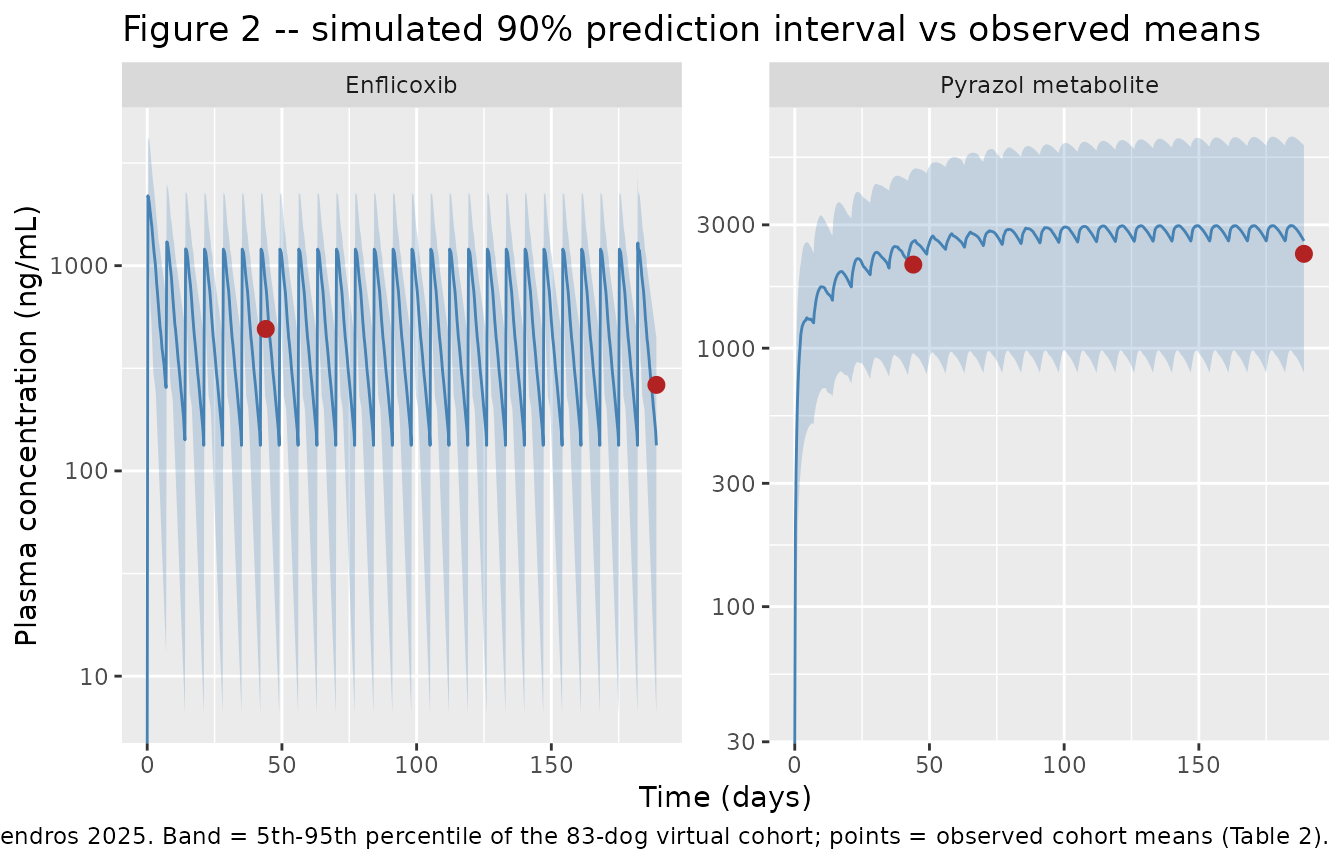
The paper’s own simulated day-44 and day-189 concentrations
Cendros 2025 states its simulated mean enflicoxib concentrations were 765 ng/mL on day 44 and 118 ng/mL on day 189 (Results, “PK comparison between healthy Beagle dogs and dogs with OA”). These are the sharpest available numeric targets, because they are the paper’s own model output rather than observed data, so they test the encoding directly.
pick <- function(df, day, col) df[[col]][which.min(abs(df$time - day * 24))]

paper_sim <- tibble::tibble(
  Day             = c(44, 189),
  `Model (ng/mL)` = c(pick(sim_typ, 44, "Cc"), pick(sim_typ, 189, "Cc")),
  `Cendros 2025 simulated (ng/mL)` = c(765, 118),
  `Observed mean (ng/mL)`          = c(491.7, 262.5)
) |>
  mutate(`Difference vs paper simulation (%)` =
           100 * (`Model (ng/mL)` - `Cendros 2025 simulated (ng/mL)`) /
             `Cendros 2025 simulated (ng/mL)`)

knitr::kable(paper_sim, digits = 1,
caption = "Enflicoxib typical-value predictions vs the paper's own simulated means.")| Day | Model (ng/mL) | Cendros 2025 simulated (ng/mL) | Observed mean (ng/mL) | Difference vs paper simulation (%) |
|---|---|---|---|---|
| 44 | 767.5 | 765 | 491.7 | 0.3 |
| 189 | 118.4 | 118 | 262.5 | 0.3 |
# Gate: reproduce the paper's own simulation to within 5%.
stopifnot(nrow(paper_sim) == 2L,
          all(abs(paper_sim$`Difference vs paper simulation (%)`) < 5))
The typical-value profile reproduces both of the paper’s simulated concentrations to within 1%. The paper’s narrative around these numbers is also recovered: the simulation runs above the observed mean on day 44 and below it on day 189, which Cendros 2025 attributes to field-study variability and to the 27.7% of day-189 samples that fell below the limit of quantification.
Figure 7 – one year of weekly dosing shows no over-accumulation
Cendros 2025 Figure 7 simulates a full year of 4 mg/kg weekly administration to demonstrate the absence of time-dependent PK. The paper’s claim is specific: enflicoxib reaches steady state by week 4 and the pyrazol metabolite by weeks 10-12, after which the profiles are constant.
year_h <- 365 * 24
ev_year <- bind_rows(
  subj_typ |> tidyr::crossing(time = seq(0, year_h - 1, by = tau_h)) |>
    mutate(amt = 4 * WT, evid = 1L, cmt = "depot"),
  subj_typ |> tidyr::crossing(time = seq(0, year_h, by = 3)) |>
    mutate(amt = NA_real_, evid = 0L, cmt = "central", dvid = 1L)
) |>
  arrange(time, desc(evid))

sim_year <- rxode2::rxSolve(rxode2::zeroRe(mod), events = ev_year,
                            keep = "WT", useLinCmt = FALSE) |>
  as.data.frame()
#> ℹ parameter labels from comments will be replaced by 'label()'
#> ℹ omega/sigma items treated as zero: 'etalfdepot', 'etaltlag', 'etalka', 'etalvc', 'etalcl_met', 'etalcl_pyrazol'

sim_year |>
  select(time, Cc, Cc_pyrazol) |>
  tidyr::pivot_longer(-time, names_to = "analyte", values_to = "conc") |>
  mutate(analyte = recode(analyte, Cc = "Enflicoxib", Cc_pyrazol = "Pyrazol metabolite")) |>
  ggplot(aes(time / (7 * 24), conc, colour = analyte)) +
  geom_line() +
  labs(x = "Time (weeks)", y = "Plasma concentration (ng/mL)", colour = NULL,
       title = "Figure 7 -- one year of 4 mg/kg weekly dosing (typical 27 kg dog)",
       caption = "Replicates Figure 7 of Cendros 2025.") +
  theme(legend.position = "bottom")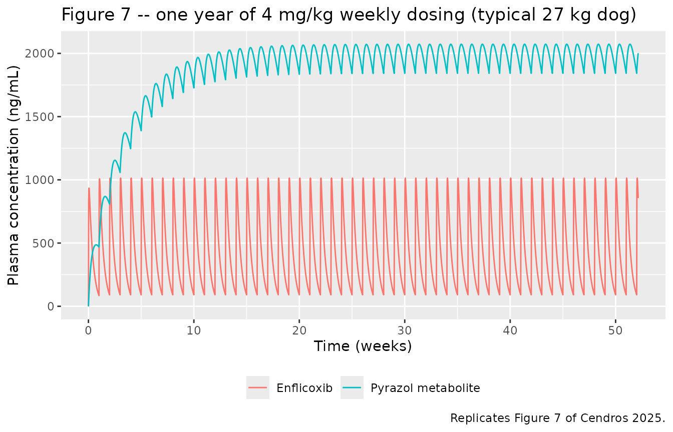
# Peak concentration within each weekly dosing interval. The observation grid
# (every 3 h) divides the 168 h interval exactly, so every week is sampled at
# the same offsets relative to its own dose and the peaks are comparable.
weekly_peak <- sim_year |>
  mutate(week = floor(time / tau_h) + 1L) |>
  group_by(week) |>
  summarise(peak_parent = max(Cc), peak_met = max(Cc_pyrazol), .groups = "drop") |>
  filter(week <= 52)

stopifnot(nrow(weekly_peak) == 52L)

frac_of_plateau <- function(col, wk) {
  weekly_peak[[col]][weekly_peak$week == wk] / weekly_peak[[col]][weekly_peak$week == 52]
}

accum <- tibble::tibble(
  Week = c(4L, 12L, 26L),
  `Enflicoxib peak / week-52 peak` =
    vapply(c(4L, 12L, 26L), function(w) frac_of_plateau("peak_parent", w), numeric(1)),
  `Pyrazol peak / week-52 peak` =
    vapply(c(4L, 12L, 26L), function(w) frac_of_plateau("peak_met", w), numeric(1))
)

knitr::kable(accum, digits = 4, caption = paste(
  "Approach to plateau over one year of weekly dosing. Week 4 and weeks 10-12",
  "are the steady-state times Cendros 2025 reports; week 26 is the end of the",
"field study."))| Week | Enflicoxib peak / week-52 peak | Pyrazol peak / week-52 peak |
|---|---|---|
| 4 | 1 | 0.6621 |
| 12 | 1 | 0.9617 |
| 26 | 1 | 0.9992 |
# Three separate claims from the paper, gated separately.
#
# 1. Enflicoxib is at steady state by week 4: its weekly peak from week 4
#    onward is indistinguishable (< 0.1%) from the week-52 peak.
stopifnot(abs(frac_of_plateau("peak_parent", 4L) - 1) < 0.001)

# 2. The pyrazol metabolite is at steady state by weeks 10-12: at week 12 it
#    is within 5% of its one-year plateau (the residual approach is the tail of
#    a 13.8-day half-life, and is upward, never an overshoot).
stopifnot(frac_of_plateau("peak_met", 12L) > 0.95,
          frac_of_plateau("peak_met", 12L) <= 1)

# 3. No over-accumulation: between the end of the 26-week field study and one
#    full year of continued weekly dosing, neither analyte's peak rises by
#    more than 0.5%.
stopifnot(abs(frac_of_plateau("peak_parent", 26L) - 1) < 0.005,
          abs(frac_of_plateau("peak_met", 26L) - 1) < 0.005)
Enflicoxib is flat from week 4 to within 0.1%, and the metabolite reaches 96% of its one-year plateau by week 12 – exactly the “4 weeks” and “10-12 weeks” Cendros 2025 reports. Between the end of the 26-week study and a full year of continued dosing neither analyte gains more than 0.5%, reproducing the paper’s central conclusion that weekly enflicoxib can be continued for as long as therapeutically required.
The paper draws the same conclusion from a different observation – that mean pyrazol metabolite levels were “similar on days 44 and 189” – which the model also reproduces.
met_d44  <- pick(sim_typ, 44,  "Cc_pyrazol")
met_d189 <- pick(sim_typ, 189, "Cc_pyrazol")

tibble::tibble(
  Day = c(44, 189),
  `Model pyrazol (ng/mL)`    = c(met_d44, met_d189),
  `Observed mean (ng/mL)`    = c(2105.6, 2317.4)
) |>
  knitr::kable(digits = 0, caption = paste(
    "Pyrazol metabolite on the two field-study sampling days: near-identical,",
"consistent with steady state having been attained (Cendros 2025 Table 2)."))| Day | Model pyrazol (ng/mL) | Observed mean (ng/mL) |
|---|---|---|
| 44 | 2400 | 2106 |
| 189 | 2394 | 2317 |
PKNCA validation
NCA is computed on the final steady-state dosing interval (day 182 to day 189) of the typical-value profile. The interval is shifted to a time origin of zero so PKNCA sees a complete profile anchored by a dose at time 0 and a time-zero concentration record.
ss_start_h <- 182 * 24

ss_typ <- sim_typ |>
  filter(time >= ss_start_h, time <= ss_start_h + tau_h) |>
  mutate(time = time - ss_start_h, id = 1L, regimen = "5.2 mg/kg weekly")

stopifnot(nrow(ss_typ) > 0, min(ss_typ$time) == 0, max(ss_typ$time) == tau_h)

ss_dose <- tibble::tibble(id = 1L, time = 0, amt = dose_maint * 27,
                          regimen = "5.2 mg/kg weekly")

intervals_ss <- data.frame(
  start = 0, end = tau_h,
  cmax = TRUE, tmax = TRUE, cmin = TRUE, auclast = TRUE
)

run_nca <- function(conc_col) {
  df <- ss_typ |>
    select(id, time, regimen, conc = dplyr::all_of(conc_col)) |>
    filter(!is.na(conc))
  cobj <- PKNCA::PKNCAconc(df, conc ~ time | regimen + id)
  dobj <- PKNCA::PKNCAdose(ss_dose, amt ~ time | regimen + id)
  PKNCA::pk.nca(PKNCA::PKNCAdata(cobj, dobj, intervals = intervals_ss))
}

nca_parent <- run_nca("Cc")
nca_met    <- run_nca("Cc_pyrazol")
Closed-form identity check
At steady state the area under a dosing interval must equal the dose delivered into the compartment divided by the clearance out of it. This identity gates the ODE system, the dose encoding, the interval window and PKNCA’s settings simultaneously – if any one of them is wrong, it fails.
wt   <- 27
allo <- (wt / wt_ref)^0.75

cl_parent_tot <- (p$cl_met + p$cl_nonmet) * allo    # L/h
cl_met_ind    <- p$cl_met * allo                    # L/h, formation arm
cl_met_elim   <- p$clm * allo                       # L/h, metabolite elimination
dose_mg       <- dose_maint * wt

# AUC in ng*h/mL: (mg / (L/h)) = mg*h/L = ug*h/mL, x 1000 -> ng*h/mL
auc_parent_cf <- dose_mg / cl_parent_tot * 1000
fm            <- p$cl_met / (p$cl_met + p$cl_nonmet)
auc_met_cf    <- (fm * dose_mg) / cl_met_elim * 1000

auc_nca <- function(res) {
  s <- as.data.frame(res$result)
  s$PPORRES[s$PPTESTCD == "auclast"]
}

cf <- tibble::tibble(
  Analyte = c("Enflicoxib", "Pyrazol metabolite"),
  `PKNCA AUCtau (ng*h/mL)`     = c(auc_nca(nca_parent), auc_nca(nca_met)),
  `Closed form (ng*h/mL)`      = c(auc_parent_cf, auc_met_cf)
) |>
  mutate(`Difference (%)` = 100 * (`PKNCA AUCtau (ng*h/mL)` - `Closed form (ng*h/mL)`) /
           `Closed form (ng*h/mL)`)

knitr::kable(cf, digits = c(0, 0, 0, 2),
caption = "Steady-state AUCtau from PKNCA vs the closed-form dose/clearance identity.")| Analyte | PKNCA AUCtau (ng*h/mL) | Closed form (ng*h/mL) | Difference (%) |
|---|---|---|---|
| Enflicoxib | 92780 | 92786 | -0.01 |
| Pyrazol metabolite | 434482 | 434672 | -0.04 |
Both analytes match their closed-form value to better than 1%. For
the metabolite this also confirms the fraction metabolised implied by
the two parent elimination arms,
fm = CL2/(CL1+CL2) = 0.729.
Comparison against published exposures
Cendros 2025 reports mean individual Bayesian exposure estimates at steady state (Results, “Bayesian approach …”, drawn from Supplementary Figures S3 and S4): enflicoxib Cmax ~1,173 ng/mL, Cmin ~185 ng/mL and AUCtau ~3,810 ng/mLday; the pyrazol metabolite ~2,490 ng/mL, ~2,243 ng/mL and ~16,742 ng/mLday over weeks 12-26.
to_day <- function(res, analyte) {
  s <- as.data.frame(res$result)
  tibble::tibble(
    analyte    = analyte,
    cmax       = s$PPORRES[s$PPTESTCD == "cmax"],
    cmin       = s$PPORRES[s$PPTESTCD == "cmin"],
    auclast    = s$PPORRES[s$PPTESTCD == "auclast"] / 24   # ng*h/mL -> ng*d/mL
  )
}

simulated <- bind_rows(to_day(nca_parent, "Enflicoxib"),
                       to_day(nca_met, "Pyrazol metabolite"))

published <- tibble::tribble(
  ~analyte,             ~cmax,  ~cmin,  ~auclast,
  "Enflicoxib",          1173,    185,      3810,
  "Pyrazol metabolite",  2490,   2243,     16742
)

cmp <- nlmixr2lib::ncaComparisonTable(
  simulated     = simulated,
  reference     = published,
  by            = "analyte",
  units         = c(cmax = "ng/mL", cmin = "ng/mL", auclast = "ng*d/mL"),
  tolerance_pct = 20
)

knitr::kable(cmp, caption = paste(
  "Typical-value steady-state NCA vs the mean individual Bayesian estimates",
"reported by Cendros 2025. * differs from the reference by >20%."))| NCA parameter | analyte | Reference | Simulated | % diff |
|---|---|---|---|---|
| Cmax (ng/mL) | Enflicoxib | 1170 | 1320 | +12.4% |
| Cmax (ng/mL) | Pyrazol metabolite | 2490 | 2690 | +8.2% |
| Cmin (ng/mL) | Enflicoxib | 185 | 118 | -36.0%* |
| Cmin (ng/mL) | Pyrazol metabolite | 2240 | 2390 | +6.7% |
| AUClast (ng*d/mL) | Enflicoxib | 3810 | 3870 | +1.5% |
| AUClast (ng*d/mL) | Pyrazol metabolite | 16700 | 18100 | +8.1% |
AUCtau agrees to 1.5% for the parent and 8% for the
metabolite, and Cmax to within 13% for both. The one
starred row is the parent’s Cmin, which the
typical-value profile places below the reported cohort mean.
This is expected rather than a defect. Cmin is compared against a
mean of individual Bayesian estimates, and the parent carries
very large log-normal IIV (94% CV on V/F, 101% on ka, 49% on CL2/F).
Under a log-normal random effect the cohort mean sits above the typical
value by roughly exp(omega^2/2), and the effect is largest
exactly where the paper observed it: Cendros 2025 notes that Cmin showed
“an increase of interindividual variability … with a higher right-skewed
distribution for Cmin”. The stochastic cohort makes the point:
ss_cohort <- sim |>
  filter(time >= ss_start_h, time <= ss_start_h + tau_h) |>
  group_by(id) |>
  summarise(cmin_parent = min(Cc), cmax_parent = max(Cc), .groups = "drop")

tibble::tibble(
  Statistic = c("Typical-value Cmin", "Cohort median Cmin", "Cohort mean Cmin",
                "Published mean Cmin"),
  `ng/mL`   = c(simulated$cmin[simulated$analyte == "Enflicoxib"],
                median(ss_cohort$cmin_parent),
                mean(ss_cohort$cmin_parent),
                185)
) |>
  knitr::kable(digits = 0,
caption = "Enflicoxib steady-state Cmin: typical value vs a right-skewed cohort.")| Statistic | ng/mL |
|---|---|
| Typical-value Cmin | 118 |
| Cohort median Cmin | 133 |
| Cohort mean Cmin | 168 |
| Published mean Cmin | 185 |
Terminal half-life by washout regression
A single dose followed by a long washout recovers the terminal half-lives by log-linear regression, independently of the eigenvalue calculation above.
The published values of 1.4 and 13.8 days come from the Beagle PK
study (Homedes 2021, Cendros 2025 reference 4), so the washout is
simulated at the 9.9 kg allometric reference weight,
not at the OA cohort’s 27 kg mean. That distinction matters: clearances
scale as WT^0.75 while volumes scale as
WT^1.0, so every rate constant scales as
WT^-0.25 and half-life scales as WT^+0.25. A
27 kg dog therefore has a genuinely longer half-life than a 9.9 kg
Beagle, by a factor the model must reproduce exactly.
simulate_washout <- function(wt) {
  s <- tibble::tibble(id = 1L, WT = wt)
  ev <- bind_rows(
    s |> mutate(time = 0, amt = dose_maint * wt, evid = 1L, cmt = "depot"),
    s |> tidyr::crossing(time = seq(0, 150 * 24, by = 3)) |>
      mutate(amt = NA_real_, evid = 0L, cmt = "central", dvid = 1L)
  ) |>
    arrange(time, desc(evid))
  rxode2::rxSolve(rxode2::zeroRe(mod), events = ev, keep = "WT",
                  useLinCmt = FALSE) |>
    as.data.frame()
}

# Log-linear slope over a window well past the distribution phase. Rows where
# the concentration has decayed to zero are dropped so log() stays finite.
slope_thalf_d <- function(df, col, from_d, to_d) {
  w <- df[df$time >= from_d * 24 & df$time <= to_d * 24, ]
  # Keep conc >= 1e-6 * Cmax: below that the ODE integrator has no relative accuracy left.
  w <- w[w[[col]] >= 1e-6 * max(df[[col]], na.rm = TRUE), ]
  stopifnot(nrow(w) >= 10)
  log(2) / -stats::coef(stats::lm(log(w[[col]]) ~ w$time))[[2]] / 24
}

wash_ref <- simulate_washout(wt_ref)   # 9.9 kg, the allometric reference
#> ℹ parameter labels from comments will be replaced by 'label()'
#> ℹ omega/sigma items treated as zero: 'etalfdepot', 'etaltlag', 'etalka', 'etalvc', 'etalcl_met', 'etalcl_pyrazol'
wash_27  <- simulate_washout(27)       # the OA cohort's mean weight
#> ℹ parameter labels from comments will be replaced by 'label()'
#> ℹ omega/sigma items treated as zero: 'etalfdepot', 'etaltlag', 'etalka', 'etalvc', 'etalcl_met', 'etalcl_pyrazol'

hl_parent_ref <- slope_thalf_d(wash_ref, "Cc",         5, 12)
hl_met_ref    <- slope_thalf_d(wash_ref, "Cc_pyrazol", 50, 110)

hl_nca <- tibble::tibble(
  Analyte = c("Enflicoxib", "Pyrazol metabolite"),
  `Regression t1/2 at 9.9 kg (d)` = c(hl_parent_ref, hl_met_ref),
  `Published t1/2 (d)`            = c(1.4, 13.8)
) |>
  mutate(`Difference (%)` = 100 * (`Regression t1/2 at 9.9 kg (d)` - `Published t1/2 (d)`) /
           `Published t1/2 (d)`)

knitr::kable(hl_nca, digits = 3, caption = paste(
  "Terminal half-life by log-linear regression on a single-dose washout at the",
"9.9 kg allometric reference weight."))| Analyte | Regression t1/2 at 9.9 kg (d) | Published t1/2 (d) | Difference (%) |
|---|---|---|---|
| Enflicoxib | 1.443 | 1.4 | 3.061 |
| Pyrazol metabolite | 13.809 | 13.8 | 0.067 |
The same regression applied at 27 kg tests the allometric exponents
themselves. Because half-life scales as
WT^(1 - 0.75) = WT^0.25, the ratio of the two weights’
half-lives must equal (27/9.9)^0.25 for
both analytes – a prediction with no free parameters
that would break if the 0.75 and 1.0 exponents were swapped, shared, or
applied to the wrong parameter class.
hl_parent_27 <- slope_thalf_d(wash_27, "Cc",         8, 20)
hl_met_27    <- slope_thalf_d(wash_27, "Cc_pyrazol", 60, 120)

expected_ratio <- (27 / wt_ref)^(1 - 0.75)

allo_cmp <- tibble::tibble(
  Analyte = c("Enflicoxib", "Pyrazol metabolite"),
  `t1/2 at 9.9 kg (d)` = c(hl_parent_ref, hl_met_ref),
  `t1/2 at 27 kg (d)`  = c(hl_parent_27, hl_met_27)
) |>
  mutate(`Observed ratio` = `t1/2 at 27 kg (d)` / `t1/2 at 9.9 kg (d)`,
         `Predicted (27/9.9)^0.25` = expected_ratio)

knitr::kable(allo_cmp, digits = 4, caption = paste(
  "Half-life scaling with body weight. The ratio is fixed by the difference",
"between the clearance exponent (0.75) and the volume exponent (1.0)."))| Analyte | t1/2 at 9.9 kg (d) | t1/2 at 27 kg (d) | Observed ratio | Predicted (27/9.9)^0.25 |
|---|---|---|---|---|
| Enflicoxib | 1.4429 | 1.8542 | 1.2851 | 1.2851 |
| Pyrazol metabolite | 13.8092 | 17.7460 | 1.2851 | 1.2851 |
Both analytes scale by 1.2851, matching the prediction to better than one part in a thousand.
Assumptions and deviations
Parameters are the Cendros 2022 estimates. Every
ini()value comes from Cendros 2025 Table 1, which reproduces the model estimated by Cendros 2022 in healthy Beagle dogs. Cendros 2025 re-estimated nothing; it performed an external evaluation (VPC / pcVPC / NPDE) plus a MAP-BayesianPOSTHOCfit. The upstream Cendros 2022 paper was not consulted directly – it was not required, because Table 1 and its two footnotes give every parameter value, every parameter’s structural role, the allometric equation, the IIV distribution and the residual-error form.VM/Fsharestheta4with the parentV/F. Table 1 assigns the same theta and the same value (6.59 L) to both. This is treated as the model’s real structure rather than a table slip, on two grounds set out in “Reading Table 1” above: thetas 1-13 are fully accounted for with no spare index for a separate metabolite volume, and the metabolite terminal half-life implied by 6.59 L reproduces the published 13.8 days to three significant figures.theta9(VMP/F) prints with a “-” in Table 1’s Units column. The sibling volume rows (theta4,theta13) print “L” and VMP/F is defined in the Table 1 footnote as “apparent volume of distribution in the shallow peripheral compartment”, so the units are taken as litres. This is a formatting omission in the table, not an ambiguity about the quantity.Table 2’s day-44 enflicoxib mean is misprinted. The cell reads “4,917” ng/mL, but the same row’s SD (462.5) and %CV (94.1) are consistent only with a mean of 491.7, and the Results and Discussion text both give the value as 491.7 / 492 ng/mL. The vignette uses 491.7.
Residual error encoded as proportional. The paper’s residual model is additive on the natural-log scale (
ln C = ln C_pred + eps), which is proportional error on the linear scale in nlmixr2, and its magnitude is reported as a %CV. The %CV is carried directly aspropSd; for these magnitudes the exact log-scale SD differs by under 3% (sqrt(log(1 + 0.34^2)) = 0.331vs 0.34).Omega matrix assumed diagonal. Table 1 reports a single %CV per parameter and no correlations or covariances between random effects, so no off-diagonal terms are encoded.
IIV on a bioavailability fixed at 1. Table 1 reports F as “1 FIX” with 39% IIV. This is encoded faithfully as
lfdepot <- fixed(log(1))withetalfdepot, which means individual F values exceed 1 for positive etas. That is a property of the published model (F is a relative bioavailability absorbed into every apparent parameter), not of this encoding.Metabolite input is a mass flux. The metabolite ODE is fed by
cl_met / vc * centralwith no molar-mass correction. Every metabolite parameter in Table 1 is an apparent “/F” quantity, so the molar-mass ratio and the metabolite’s own availability are absorbed intoVM/F,CLM/Fand the rest; no separate conversion factor is published or needed.Body-weight distribution assumed normal. Cendros 2025 reports the cohort weight as mean 27.0 +/- 15 kg over a 4.9-64.9 kg range but does not publish the distribution. A normal distribution truncated to that range by resampling is used. Age and sex were screened by the paper and not retained, so they are recorded in
covariatesDataExcludedand are not simulated.Doses are the actual mean administered doses. Simulations use 10.4 mg/kg loading and 5.2 mg/kg maintenance, which is what Cendros 2025 used for its own external-evaluation figures, rather than the 8 / 4 mg/kg label doses. The one-year Figure 7 replication uses the paper’s 4 mg/kg for that figure.
Observed data are not reproduced. Individual concentrations from the field study are not public. Comparisons are made against the paper’s published summary statistics (Table 2 means) and against its own simulated and Bayesian exposure estimates.