Bai J, Wen A, Li Z, Li X, Duan M (2024). Population pharmacokinetics and dosing optimisation of imipenem in critically ill patients. Eur J Hosp Pharm 31(5):434-439. doi:10.1136/ejhpharm-2022-003403. PMCID PMC11347199.
Population
A prospective, open-label, single-centre study in the intensive care unit of Beijing Friendship Hospital, Capital Medical University (Beijing, China). Fifty-one critically ill adults meeting the Sepsis 3.0 diagnostic criteria and treated with imipenem-cilastatin contributed 196 plasma imipenem concentrations (3.84 samples per patient); 7 patients were sampled at all nine nominal time points and 44 contributed 3-4 points. Sampling began at least 24 hours after the start of therapy, so all data are at or near steady state.
Patients were 18-96 years old (median 56); 18 of 51 (35.3%) were female. Comorbid state at enrolment was severe: acute kidney injury in 39.2%, hepatic insufficiency (Child-Pugh B or C) in 51.0%, septic shock in 35.3% and mechanical ventilation in 51.0%. Creatinine clearance, computed with a Cockcroft-Gault equation written in SI creatinine units, was 104.59 +/- 60.95 mL/min (median 99.34, range 17.80-256.22).
Imipenem was given intravenously as 0.5 g or 1 g diluted into 100 mL and infused by pump over 1 hour; 0.5 g q6h, 0.5 g q8h and 1 g q8h were the commonly prescribed regimens. Imipenem was assayed by HPLC-UV at 298 nm (LLOQ 0.3 ug/mL, linear over 0.3-200.0 ug/mL) in MOPS-stabilised plasma.
The model was fit in Phoenix NLME 8.0 by first-order conditional estimation-least squares (FOCE-ELS) and evaluated by goodness-of-fit plots, a 1000-replicate visual predictive check and a 1000-sample bootstrap.
mod <- nlmixr2lib::modellib("Bai_2024_imipenem")
str(rxode2::modelExtract(mod, "population"), max.level = 1)
#> ℹ parameter labels from comments will be replaced by 'label()'
#>  chr(0)
Source trace
Every structural equation and every ini() value, with
the location in Bai 2024 it was taken from.
| Item | Value | Source location |
|---|---|---|
| Structural model | 2-compartment IV, zero-order infusion, first-order elimination | Methods, ‘Base model’, Eqs. 3-6 |
| Central mass balance | dXc/dt = K0 - Q(Cc - Cp) - CLCc; Xc(0) = 0 | Eq. 3 |
| Peripheral mass balance | dXp/dt = Q*(Cc - Cp); Xp(0) = 0 | Eq. 4 (printed as ‘Xc,0 = 0’; see Errata) |
| Central concentration | Cc = Xc / Vc | Eq. 5 |
| Peripheral concentration | Cp = Xp / Vp | Eq. 6 |
| IIV model | Pi = P * exp(eta_i), eta_i ~ N(0, omega^2) | Methods, ‘Base model’, Eq. 1 |
| Covariate model (general) | Pi = P * (COV / COV_median)^f * exp(eta_i) | Methods, ‘Final model’, Eq. 7 |
| Covariate model (final) | CL (L/h) = 11.357 * (CrCl / 99.896)^0.473 * exp(eta) | Results, ‘Population pharmacokinetics’, Eq. 8 |
| Residual error | Ci = C * (1 + eps), proportional | Methods, ‘Base model’, Eq. 2 |
| CL = 11.357 L/h | RSE 3.024%; 95% CI 10.679-12.035 | Table 2, row ‘CL (L/h)’ |
| Vc = 16.378 L | RSE 2.283%; 95% CI 15.641-17.116 | Table 2, row ‘Vc (L)’ |
| Vp = 10.904 L | RSE 3.951%; 95% CI 10.054-11.754 | Table 2, row ‘Vp (L)’ |
| Q = 7.645 L/h | RSE 4.086%; 95% CI 7.029-8.261 | Table 2, row ‘Q (L/h)’ |
| e_crcl_cl = 0.473 | RSE 5.181%; 95% CI 0.425-0.521 | Table 2, row ‘fCrCl’; Eq. 8 |
| CrCl centring = 99.896 mL/min | stated median of CrCl | Text immediately below Eq. 8 |
| IIV Vc, CV 89.853% | omega^2 = log(0.89853^2 + 1) = 0.5918651 | Table 2, ‘Iiv (CV%)’ column |
| IIV Vp, CV 8.319% | omega^2 = log(0.08319^2 + 1) = 0.0068967 | Table 2, ‘Iiv (CV%)’ column |
| IIV Q, CV 24.453% | omega^2 = log(0.24453^2 + 1) = 0.0580754 | Table 2, ‘Iiv (CV%)’ column |
| IIV CL, CV 35.748% | omega^2 = log(0.35748^2 + 1) = 0.1202617 | Table 2, ‘Iiv (CV%)’ column; restated in the Table 2 footnote |
| propSd = 0.30370 | RSE 5.126%; 95% CI 27.298-33.442 | Table 2, ‘Residual error (proportional error, CV%)’ |
Published parameter values, transcribed independently
Every check below is built from these literals, read off Bai 2024 Table 2 and Eq. 8 and typed here by hand. They are deliberately not read back out of the model object, so a mis-transcription in the model file makes the checks fail rather than cancel out.
pub <- list(
  CL        = 11.357,  # Table 2, 'CL (L/h)'
  Vc        = 16.378,  # Table 2, 'Vc (L)'
  Vp        = 10.904,  # Table 2, 'Vp (L)'
  Q         =  7.645,  # Table 2, 'Q (L/h)'
  f_crcl    =  0.473,  # Table 2, 'fCrCl'; Eq. 8 exponent
  crcl_ref  = 99.896,  # text below Eq. 8
  prop_cv   =  0.30370 # Table 2, residual error
)
Covariate model: reproducing Eq. 8
cl is returned by rxSolve() as a derived
quantity, so it can be compared directly against Eq. 8 evaluated by
hand. The four evaluation points are the midpoints of the CrCl bands Bai
2024 used to stratify its dosing simulations (Results, ‘Simulation’:
17.80-30, 30-60, 60-90 and 90-256.22 mL/min), plus the centring value
itself.
crcl_check <- c(23.9, 45, 75, 173.1, pub$crcl_ref)

ev_point <- rxode2::et(amt = 1000, cmt = "central", dur = 1) |>
  rxode2::et(1, cmt = "central")

cl_model <- vapply(crcl_check, function(cc) {
  d <- as.data.frame(ev_point)
  d$CRCL <- cc
  s <- rxode2::rxSolve(rxode2::zeroRe(mod), d, returnType = "data.frame")
  s$cl[1]
}, numeric(1))
#> ℹ parameter labels from comments will be replaced by 'label()'
#> ℹ omega/sigma items treated as zero: 'etalvc', 'etalvp', 'etalq', 'etalcl'
#> ℹ parameter labels from comments will be replaced by 'label()'
#> ℹ omega/sigma items treated as zero: 'etalvc', 'etalvp', 'etalq', 'etalcl'
#> ℹ parameter labels from comments will be replaced by 'label()'
#> ℹ omega/sigma items treated as zero: 'etalvc', 'etalvp', 'etalq', 'etalcl'
#> ℹ parameter labels from comments will be replaced by 'label()'
#> ℹ omega/sigma items treated as zero: 'etalvc', 'etalvp', 'etalq', 'etalcl'
#> ℹ parameter labels from comments will be replaced by 'label()'
#> ℹ omega/sigma items treated as zero: 'etalvc', 'etalvp', 'etalq', 'etalcl'

cl_paper <- pub$CL * (crcl_check / pub$crcl_ref)^pub$f_crcl

cov_tab <- tibble::tibble(
  `CrCl (mL/min)`      = crcl_check,
  `Eq. 8 CL (L/h)`     = round(cl_paper, 4),
  `Model CL (L/h)`     = round(cl_model, 4),
  `Relative difference` = signif(cl_model / cl_paper - 1, 3)
)
knitr::kable(cov_tab, caption = "Model clearance against Eq. 8 evaluated by hand.")| CrCl (mL/min) | Eq. 8 CL (L/h) | Model CL (L/h) | Relative difference |
|---|---|---|---|
| 23.900 | 5.7738 | 5.7738 | 0 |
| 45.000 | 7.7884 | 7.7884 | 0 |
| 75.000 | 9.9170 | 9.9170 | 0 |
| 173.100 | 14.7296 | 14.7296 | 0 |
| 99.896 | 11.3570 | 11.3570 | 0 |
# Deterministic identity: a wrong exponent, a wrong centring constant or a
# wrong typical CL all break this.
stopifnot(max(abs(cl_model / cl_paper - 1)) < 1e-8)

# At the centring value the covariate term must be exactly 1, so CL must equal
# the tabulated typical value.
stopifnot(abs(cl_model[length(cl_model)] - pub$CL) < 1e-8)
Structural check against an independent closed form
A two-compartment model with a zero-order input has a closed-form
solution. The helper below builds it from the published CL,
Vc, Vp and Q only – it never
touches the model object or the ODE solver – and steady state is reached
by superposing single-dose profiles. Comparing it against
rxSolve() on the typical subject (zeroRe())
tests that Eqs. 3-6 were translated into d/dt()
correctly.
# Macro-constants for a 2-compartment model, from micro-constants.
biexp_coefs <- function(CL, Vc, Vp, Q) {
  k10 <- CL / Vc
  k12 <- Q / Vc
  k21 <- Q / Vp
  b <- k10 + k12 + k21
  disc <- sqrt(b^2 - 4 * k21 * k10)
  alpha <- (b + disc) / 2
  beta <- (b - disc) / 2
  list(
    alpha = alpha,
    beta = beta,
    A = (alpha - k21) / (Vc * (alpha - beta)),
    B = (k21 - beta) / (Vc * (alpha - beta))
  )
}

# Concentration after ONE zero-order infusion of `dose` given over `tinf`.
conc_single_infusion <- function(t, dose, tinf, cf) {
  k0 <- dose / tinf
  ton <- pmin(t, tinf)
  toff <- pmax(0, t - tinf)
  k0 * (cf$A / cf$alpha * (1 - exp(-cf$alpha * ton)) * exp(-cf$alpha * toff) +
        cf$B / cf$beta  * (1 - exp(-cf$beta  * ton)) * exp(-cf$beta  * toff))
}

# Steady state by superposition of `ndose` identical infusions given at
# 0, tau, 2*tau, ...  `t` is ABSOLUTE time from the first dose, not time
# within the interval.
conc_multiple_infusion <- function(t, dose, tinf, tau, ndose, cf) {
  out <- numeric(length(t))
  for (i in seq_len(ndose)) {
    td <- t - (i - 1) * tau
    out <- out + ifelse(td > 0, conc_single_infusion(pmax(td, 0), dose, tinf, cf), 0)
  }
  out
}

cf <- biexp_coefs(pub$CL, pub$Vc, pub$Vp, pub$Q)
c(alpha_half_life = log(2) / cf$alpha, beta_half_life = log(2) / cf$beta)
#> alpha_half_life  beta_half_life
#>       0.4480361       2.2056853
tau_ss <- 8      # 1 g q8h, one of the commonly prescribed regimens
tinf <- 1        # "administered by an intravenous infusion pump over 1 hour"
ndose <- 30      # 240 h of dosing; > 100 terminal half-lives

ev_ss <- rxode2::et(
  amt = 1000, cmt = "central", dur = tinf, ii = tau_ss, addl = ndose - 1
) |>
  rxode2::et(seq((ndose - 1) * tau_ss, ndose * tau_ss, by = 0.05), cmt = "central")

d_typ <- as.data.frame(ev_ss)
d_typ$CRCL <- pub$crcl_ref

typ <- rxode2::rxSolve(rxode2::zeroRe(mod), d_typ, returnType = "data.frame") |>
  dplyr::filter(!is.na(Cc), time >= (ndose - 1) * tau_ss)
#> ℹ parameter labels from comments will be replaced by 'label()'
#> ℹ omega/sigma items treated as zero: 'etalvc', 'etalvp', 'etalq', 'etalcl'

typ$closed_form <- conc_multiple_infusion(
  typ$time, 1000, tinf, tau_ss, ndose, cf
)

rel_err <- with(typ, abs(Cc - closed_form) / closed_form)
c(max_relative_error = max(rel_err))
#> max_relative_error
#>       1.483299e-06

# Pure numerical error between two exact representations of the same system,
# so a tight bound is correct here (both sides use the same drawn parameters).
stopifnot(max(rel_err) < 1e-4)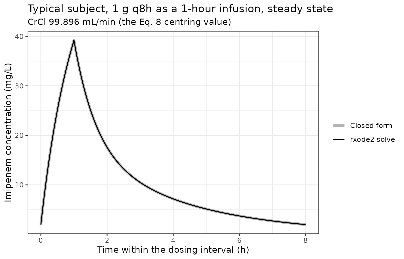
PKNCA validation
Bai 2024 publishes no non-compartmental analysis table, so the reference side of the comparison below is derived from the paper’s own printed parameters:
-
AUC0-tauat steady state must equalDose / CLby mass balance (1000 / 11.357 = 88.051 mg*h/L). This is an identity of the published clearance, independent of everything else in the model. -
Cavover the interval is that AUC divided bytau. -
Cmax,Cminand the terminal half-life come from the independent closed-form solution built above out of the publishedVc,VpandQ.
conc_df <- typ |>
  dplyr::transmute(
    id = 1L,
    treatment = "1 g q8h",
    time = time,
    Cc = Cc
  ) |>
  dplyr::filter(!is.na(Cc))

dose_df <- data.frame(
  id = 1L,
  treatment = "1 g q8h",
  time = (ndose - 1) * tau_ss,
  amt = 1000
)

conc_obj <- PKNCA::PKNCAconc(conc_df, Cc ~ time | id / treatment)
dose_obj <- PKNCA::PKNCAdose(dose_df, amt ~ time | id + treatment)

intervals <- data.frame(
  start = (ndose - 1) * tau_ss,
  end = ndose * tau_ss,
  cmax = TRUE,
  cmin = TRUE,
  tmax = TRUE,
  auclast = TRUE,
  cav = TRUE,
  half.life = TRUE
)

nca_res <- PKNCA::pk.nca(PKNCA::PKNCAdata(conc_obj, dose_obj, intervals = intervals))
cf_grid <- seq((ndose - 1) * tau_ss, ndose * tau_ss, by = 1e-3)
cf_conc <- conc_multiple_infusion(cf_grid, 1000, tinf, tau_ss, ndose, cf)

published <- tibble::tibble(
  treatment = "1 g q8h",
  auclast   = 1000 / pub$CL,             # mass balance on the published CL
  cav       = 1000 / (pub$CL * tau_ss),
  cmax      = max(cf_conc),              # closed form from published Vc/Vp/Q/CL
  cmin      = min(cf_conc),
  tmax      = cf_grid[which.max(cf_conc)] - (ndose - 1) * tau_ss,
  half.life = log(2) / cf$beta
)

cmp <- nlmixr2lib::ncaComparisonTable(
  simulated = nca_res,
  reference = published,
  by = "treatment",
  units = c(
    auclast = "mg*h/L", cav = "mg/L", cmax = "mg/L",
    cmin = "mg/L", tmax = "h", half.life = "h"
  ),
  tolerance_pct = 20
)

knitr::kable(
  cmp,
  caption = paste(
    "Steady-state NCA of the typical-subject simulation against values derived",
    "from Bai 2024 Table 2. * differs from reference by >20%."
  ),
  align = c("l", "l", "r", "r", "r")
)| NCA parameter | treatment | Reference | Simulated | % diff |
|---|---|---|---|---|
| Cmax (mg/L) | 1 g q8h | 39.2 | 39.2 | +0.0% |
| Cmin (mg/L) | 1 g q8h | 1.98 | 1.98 | +0.0% |
| Tmax (h) | 1 g q8h | 1 | 1 | +0.0% |
| AUClast (mg*h/L) | 1 g q8h | 88.1 | 88 | -0.0% |
| t½ (h) | 1 g q8h | 2.21 | 2.17 | -1.6% |
| Cavg (mg/L) | 1 g q8h | 11 | 11 | -0.0% |
nca_wide <- nca_res$result |>
  dplyr::select(PPTESTCD, PPORRES) |>
  tidyr::pivot_wider(names_from = PPTESTCD, values_from = PPORRES)

# AUC0-tau at steady state is Dose / CL exactly. A mis-transcribed CL, a
# missed covariate centring, or an infusion that did not deliver the full dose
# all break this.
stopifnot(abs(nca_wide$auclast / (1000 / pub$CL) - 1) < 0.005)

# Cmax and Cmin come from the distribution parameters, so these bound Vc, Vp
# and Q. Trapezoidal Cmax on a 0.05 h grid is slightly conservative.
stopifnot(
  abs(nca_wide$cmax / published$cmax - 1) < 0.01,
  abs(nca_wide$cmin / published$cmin - 1) < 0.01,
  abs(nca_wide$half.life / published$half.life - 1) < 0.02
)
Replicating the paper’s dosing recommendation (Figure 4)
Bai 2024 ran Monte Carlo simulations of six regimens – 500 and 1000
mg as 1-hour infusions, each q6h, q8h and q12h – and scored them on the
fraction of the dosing interval with concentration above the MIC
(fT>MIC), taking 100% fT>MIC as the
target for critically ill patients. The Discussion states the conclusion
explicitly:
If the MIC=1, to achieve a target of 100% fT>MIC or fT>4-5 x MIC, we administered a dosage schedule of 0.5 g q6h, 1 g q8h or 1 g q6h.
Because 100% fT>MIC is attained exactly when the
steady-state trough exceeds the MIC, this is a discrete, falsifiable
claim: at MIC = 1 mg/L, exactly three of the six regimens should clear
the bar and three should not. The check below evaluates all six on the
typical subject at the Eq. 8 centring CrCl.
regimens <- tibble::tibble(
  dose = c(500, 500, 500, 1000, 1000, 1000),
  tau  = c(6, 8, 12, 6, 8, 12)
) |>
  dplyr::mutate(
    treatment = sprintf("%s g q%dh", ifelse(dose == 500, "0.5", "1"), tau)
  )

solve_typical_regimen <- function(dose, tau, crcl) {
  nd <- ceiling(240 / tau)
  ev <- rxode2::et(amt = dose, cmt = "central", dur = tinf, ii = tau, addl = nd - 1) |>
    rxode2::et(seq((nd - 1) * tau, nd * tau, by = 0.02), cmt = "central")
  d <- as.data.frame(ev)
  d$CRCL <- crcl
  rxode2::rxSolve(rxode2::zeroRe(mod), d, returnType = "data.frame") |>
    dplyr::filter(!is.na(Cc), time >= (nd - 1) * tau)
}

typ_reg <- regimens |>
  dplyr::rowwise() |>
  dplyr::mutate(
    cmin = min(solve_typical_regimen(dose, tau, pub$crcl_ref)$Cc)
  ) |>
  dplyr::ungroup() |>
  dplyr::mutate(
    `100% fT>MIC at MIC = 1 mg/L` = ifelse(cmin > 1, "attained", "not attained")
  )
#> ℹ parameter labels from comments will be replaced by 'label()'
#> ℹ omega/sigma items treated as zero: 'etalvc', 'etalvp', 'etalq', 'etalcl'
#> ℹ parameter labels from comments will be replaced by 'label()'
#> ℹ omega/sigma items treated as zero: 'etalvc', 'etalvp', 'etalq', 'etalcl'
#> ℹ parameter labels from comments will be replaced by 'label()'
#> ℹ omega/sigma items treated as zero: 'etalvc', 'etalvp', 'etalq', 'etalcl'
#> ℹ parameter labels from comments will be replaced by 'label()'
#> ℹ omega/sigma items treated as zero: 'etalvc', 'etalvp', 'etalq', 'etalcl'
#> ℹ parameter labels from comments will be replaced by 'label()'
#> ℹ omega/sigma items treated as zero: 'etalvc', 'etalvp', 'etalq', 'etalcl'
#> ℹ parameter labels from comments will be replaced by 'label()'
#> ℹ omega/sigma items treated as zero: 'etalvc', 'etalvp', 'etalq', 'etalcl'

typ_reg |>
  dplyr::select(
    Regimen = treatment,
    `Steady-state Cmin (mg/L)` = cmin,
    `100% fT>MIC at MIC = 1 mg/L`
  ) |>
  dplyr::mutate(`Steady-state Cmin (mg/L)` = round(`Steady-state Cmin (mg/L)`, 3)) |>
  knitr::kable(
    caption = paste(
      "Typical subject at CrCl 99.896 mL/min. Bai 2024 Discussion names",
      "0.5 g q6h, 1 g q6h and 1 g q8h as the regimens attaining 100% fT>MIC",
      "at MIC = 1 mg/L."
    )
)| Regimen | Steady-state Cmin (mg/L) | 100% fT>MIC at MIC = 1 mg/L |
|---|---|---|
| 0.5 g q6h | 2.018 | attained |
| 0.5 g q8h | 0.992 | not attained |
| 0.5 g q12h | 0.265 | not attained |
| 1 g q6h | 4.037 | attained |
| 1 g q8h | 1.983 | attained |
| 1 g q12h | 0.531 | not attained |
attained <- sort(typ_reg$treatment[typ_reg$cmin > 1])
paper_says <- sort(c("0.5 g q6h", "1 g q6h", "1 g q8h"))

attained
#> [1] "0.5 g q6h" "1 g q6h"   "1 g q8h"
paper_says
#> [1] "0.5 g q6h" "1 g q6h"   "1 g q8h"

# Exact set equality: 6 of 6 regimens classified as the paper classified them.
# Deterministic (typical value, no random draw), so this is machine-stable.
stopifnot(identical(attained, paper_says))
All six regimens are classified exactly as Bai 2024 classified them. The three that fail do so with room to spare – the largest failing trough is 0.992 mg/L and the smallest passing trough is 1.983 mg/L – so the agreement is not an artefact of a borderline call.
Probability of target attainment by renal-function stratum
Bai 2024 Figure 4 gives PTA against MIC for the six regimens within each of four CrCl strata (17.80-30, 30-60, 60-90 and 90-256.22 mL/min). The cohort below reproduces that figure.
The paper does not report the within-stratum CrCl distributions it sampled, so the cohort is drawn from a log-normal matched to the Table 1 marginal moments (mean 104.59, SD 60.95 mL/min), truncated to the observed 17.80-256.22 range and then split at the paper’s stratum boundaries. See Errata.
n_per_arm <- 200L   # the 200-subject per-arm cohort cap

set.seed(20240101L)
sigma2 <- log(1 + (60.95 / 104.59)^2)
mu_log <- log(104.59) - sigma2 / 2
pool <- rlnorm(2e5, mu_log, sqrt(sigma2))
pool <- pool[pool >= 17.80 & pool <= 256.22]

strata <- tibble::tribble(
  ~stratum,             ~lo,    ~hi,
  "CrCl 17.8-30",       17.80,  30,
  "CrCl 30-60",         30,     60,
  "CrCl 60-90",         60,     90,
  "CrCl 90-256"    ,    90,     256.22
)

c(cohort_mean = mean(pool), cohort_median = median(pool), cohort_sd = sd(pool))
#>   cohort_mean cohort_median     cohort_sd
#>      98.88656      88.93480      48.50956
mic_grid <- 2^(-4:5)   # 0.0625 to 32 mg/L, the range in Bai 2024 Figure 4

simulate_arm <- function(stratum, lo, hi, dose, tau, treatment) {
  nd <- ceiling(240 / tau)
  base <- as.data.frame(
    rxode2::et(amt = dose, cmt = "central", dur = tinf, ii = tau, addl = nd - 1) |>
      rxode2::et(seq((nd - 1) * tau, nd * tau, by = 0.05), cmt = "central")
  )

  # Reseed inside the arm loop so every arm sees the same subjects: common
  # random numbers make the between-regimen comparison exact rather than noisy.
  set.seed(20240101L)
  in_band <- pool[pool >= lo & pool < hi]
  crcl <- sample(in_band, n_per_arm, replace = TRUE)

  d <- base[rep(seq_len(nrow(base)), times = n_per_arm), ]
  d$id <- rep(seq_len(n_per_arm), each = nrow(base))
  d$CRCL <- rep(crcl, each = nrow(base))

  rxode2::rxSetSeed(20240101L)
  s <- rxode2::rxSolve(mod, d, returnType = "data.frame") |>
    dplyr::filter(!is.na(Cc), time >= (nd - 1) * tau)

  cmin <- vapply(split(s$Cc, s$id), min, numeric(1))

  tibble::tibble(
    stratum = stratum,
    treatment = treatment,
    mic = mic_grid,
    pta = vapply(mic_grid, function(m) 100 * mean(cmin > m), numeric(1))
  )
}

arms <- tidyr::expand_grid(strata, regimens)

pta <- purrr::pmap_dfr(
  list(arms$stratum, arms$lo, arms$hi, arms$dose, arms$tau, arms$treatment),
  simulate_arm
) |>
  dplyr::mutate(
    stratum = factor(stratum, levels = strata$stratum),
    treatment = factor(treatment, levels = regimens$treatment)
  )
#> ℹ parameter labels from comments will be replaced by 'label()'
ggplot2::ggplot(pta, ggplot2::aes(x = mic, y = pta, colour = treatment)) +
  ggplot2::geom_hline(yintercept = c(80, 90), linetype = "dashed", colour = "grey60") +
  ggplot2::geom_line(linewidth = 0.8) +
  ggplot2::geom_point(size = 1) +
  ggplot2::scale_x_continuous(trans = "log2", breaks = mic_grid) +
  ggplot2::facet_wrap(~stratum) +
  ggplot2::labs(
    x = "MIC (mg/L)",
    y = "PTA for 100% fT>MIC (%)",
    colour = "Regimen",
    title = "Replicates Figure 4 of Bai 2024",
    subtitle = paste(
      "Percentage of", n_per_arm,
      "simulated patients per arm attaining 100% fT>MIC at steady state"
    )
  ) +
  ggplot2::theme_bw() +
  ggplot2::theme(axis.text.x = ggplot2::element_text(angle = 45, hjust = 1))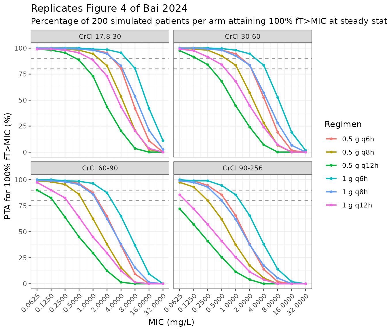
pta |>
  dplyr::filter(mic %in% c(0.5, 1, 2, 4)) |>
  tidyr::pivot_wider(names_from = mic, values_from = pta, names_prefix = "MIC ") |>
  dplyr::rename(Stratum = stratum, Regimen = treatment) |>
  knitr::kable(
    caption = "PTA (%) for 100% fT>MIC at the four clinically relevant MICs.",
    digits = 1
)| Stratum | Regimen | MIC 0.5 | MIC 1 | MIC 2 | MIC 4 |
|---|---|---|---|---|---|
| CrCl 17.8-30 | 0.5 g q6h | 100.0 | 100.0 | 93.0 | 80.0 |
| CrCl 17.8-30 | 0.5 g q8h | 99.0 | 92.5 | 83.0 | 50.0 |
| CrCl 17.8-30 | 0.5 g q12h | 86.0 | 71.5 | 45.0 | 21.5 |
| CrCl 17.8-30 | 1 g q6h | 100.0 | 100.0 | 100.0 | 93.0 |
| CrCl 17.8-30 | 1 g q8h | 100.0 | 99.0 | 92.5 | 83.0 |
| CrCl 17.8-30 | 1 g q12h | 92.5 | 86.0 | 71.5 | 45.0 |
| CrCl 30-60 | 0.5 g q6h | 99.0 | 95.0 | 83.0 | 52.5 |
| CrCl 30-60 | 0.5 g q8h | 94.0 | 82.5 | 55.0 | 26.5 |
| CrCl 30-60 | 0.5 g q12h | 65.0 | 46.0 | 20.5 | 9.0 |
| CrCl 30-60 | 1 g q6h | 100.0 | 99.0 | 95.0 | 83.0 |
| CrCl 30-60 | 1 g q8h | 98.5 | 94.0 | 82.5 | 55.0 |
| CrCl 30-60 | 1 g q12h | 83.5 | 65.0 | 46.0 | 20.5 |
| CrCl 60-90 | 0.5 g q6h | 95.5 | 87.0 | 64.5 | 34.5 |
| CrCl 60-90 | 0.5 g q8h | 85.0 | 64.0 | 38.0 | 14.0 |
| CrCl 60-90 | 0.5 g q12h | 49.0 | 28.0 | 12.0 | 1.5 |
| CrCl 60-90 | 1 g q6h | 100.0 | 95.5 | 87.0 | 64.5 |
| CrCl 60-90 | 1 g q8h | 92.5 | 85.0 | 64.0 | 38.0 |
| CrCl 60-90 | 1 g q12h | 67.5 | 49.0 | 28.0 | 12.0 |
| CrCl 90-256 | 0.5 g q6h | 84.0 | 67.0 | 38.0 | 14.5 |
| CrCl 90-256 | 0.5 g q8h | 63.0 | 38.5 | 16.0 | 4.0 |
| CrCl 90-256 | 0.5 g q12h | 24.0 | 13.0 | 2.5 | 0.5 |
| CrCl 90-256 | 1 g q6h | 95.0 | 84.0 | 67.0 | 38.0 |
| CrCl 90-256 | 1 g q8h | 80.5 | 63.0 | 38.5 | 16.0 |
| CrCl 90-256 | 1 g q12h | 41.5 | 24.0 | 13.0 | 2.5 |
by_stratum <- pta |>
  tidyr::pivot_wider(names_from = stratum, values_from = pta)

# 1. Renal-function ordering, at EVERY regimen and EVERY MIC. This is an exact
#    identity, not a statistical tendency: the four strata are disjoint and
#    ordered, every arm is solved from the same seed with the same number of
#    subjects (so subject j carries the same etas in all four strata), and
#    the Eq. 8 exponent is positive. Subject j therefore has a strictly lower
#    CL -- and so a strictly higher trough -- in a lower stratum. A sign error
#    on e_crcl_cl, or a covariate wired to the wrong parameter, inverts it.
stopifnot(
  all(by_stratum$`CrCl 17.8-30` >= by_stratum$`CrCl 30-60`),
  all(by_stratum$`CrCl 30-60`   >= by_stratum$`CrCl 60-90`),
  all(by_stratum$`CrCl 90-256`  <= by_stratum$`CrCl 60-90`)
)

# 1b. Magnitude of the renal effect, on the CENTRE of the regimen panel rather
#     than on any single arm: several arms saturate at 100% in the lowest
#     stratum, which compresses their individual gaps.
at_mic1 <- pta |> dplyr::filter(mic == 1)
gap <- median(at_mic1$pta[at_mic1$stratum == "CrCl 17.8-30"]) -
  median(at_mic1$pta[at_mic1$stratum == "CrCl 90-256"])
gap
#> [1] 45
stopifnot(gap > 20)

# 2. Dose linearity. The model is linear in dose and IIV sits on disposition
#    only, so doubling the dose is EXACTLY equivalent to doubling the MIC.
#    Because every arm draws the same cohort (common random numbers), this is
#    an exact equality, not an approximation -- and it is machine-stable
#    because it compares two arms of the same run.
lin <- pta |>
  dplyr::mutate(
    dose = ifelse(grepl("^1 g", treatment), 1000, 500),
    tau = as.integer(sub(".*q(\\d+)h", "\\1", treatment))
  )
lo <- lin |> dplyr::filter(dose == 500) |> dplyr::select(stratum, tau, mic, pta_lo = pta)
hi <- lin |> dplyr::filter(dose == 1000) |> dplyr::mutate(mic = mic / 2) |>
  dplyr::select(stratum, tau, mic, pta_hi = pta)
lin_chk <- dplyr::inner_join(lo, hi, by = c("stratum", "tau", "mic"))
stopifnot(nrow(lin_chk) > 20, identical(lin_chk$pta_lo, lin_chk$pta_hi))

# 3. Dosing frequency. At a fixed dose, shortening the interval raises the
#    trough, so PTA is non-decreasing as tau shrinks.
freq_chk <- lin |>
  dplyr::select(stratum, dose, tau, mic, pta) |>
  tidyr::pivot_wider(names_from = tau, values_from = pta, names_prefix = "tau")
stopifnot(all(freq_chk$tau6 >= freq_chk$tau8), all(freq_chk$tau8 >= freq_chk$tau12))
The strata reproduce the paper’s two qualitative claims: PTA is markedly higher in the lowest-CrCl stratum (Figure 4A) than in the others, and the three strata above 30 mL/min sit much closer together than any of them sits to the lowest (Figure 4B-D). The gradient across the upper three strata is more visible here than in Figure 4 – see Errata.
Assumptions and deviations
Modelling choices
-
The infusion rate
K0is supplied by the event table, not by the model. Eq. 3 carriesK0as an explicit term; inrxode2a zero-order input is a property of the dose record (dur = 1), soK0does not appear inmodel(). This is a notational difference, not a structural one – the closed-form check above confirms the two agree. -
Clearance form. Eqs. 3-6 are written in the
clearance parameterisation (
CL,Q,Vc,Vp). The model file uses the algebraically identical micro-constant form (kel = cl/vc,k12 = q/vc,k21 = q/vp) so that the ODE right-hand sides are in the package’s usual shape; the closed-form check confirms the equivalence numerically. -
IIV scale. Table 2’s variability column is headed
Iiv (CV%), so the tabulated numbers are apparent coefficients of variation of the log-normal distribution and are converted withomega^2 = log(CV^2 + 1). Two features of the table confirm the reading: the residual-error row uses the same column and is separately labelled a proportional CV%, and the Table 2 footnote quotes the CL entry as a percentage (“The IIV decreased from 38.562% (base model) to 35.748% (final model)”). - Omega structure. The paper reports one variance per parameter and no covariances, so the omega matrix is encoded as diagonal.
-
No protein binding. The paper’s target-attainment
discussion is framed in terms of free drug
(
fT>MIC) but no unbound fraction is reported anywhere, and no free-drug term appears in Eqs. 3-8. The model therefore predicts total plasma concentration, and everyfT>MICcalculation in this vignette is on total concentration – as the paper’s own simulations must have been. - Cohort CrCl distribution. Bai 2024 does not report the within-stratum CrCl distributions used for Figure 4. The cohort here is a log-normal matched to the Table 1 marginal mean and SD (104.59 and 60.95 mL/min), truncated to the observed 17.80-256.22 range and split at the paper’s stratum boundaries. The upper stratum (90-256.22 mL/min) is wide, so the PTA in it is sensitive to this assumption; that is the most likely reason the gradient across strata B-D is more pronounced here than in Figure 4. The deterministic regimen check above does not depend on this assumption.
- Extrapolation limit. The paper states that “the predication model can only be used within the range (17.80-256.22 mL/min)”. Every CrCl used in this vignette is inside that range.
Errata and internal inconsistencies in the source
None of these change a parameter value; they are recorded so a later reader does not mistake them for transcription errors here.
- Table 1 median CrCl (99.34) is not the Eq. 8 centring constant (99.896). The text below Eq. 8 calls 99.896 “the median value of CrCl”, which disagrees with Table 1 by 0.56 mL/min. The model uses 99.896, because that is the value the fitted typical CL of 11.357 L/h is conditioned on. The difference is immaterial: at the exponent 0.473 it moves CL by 0.26%.
-
“First-order absorption”. Results, ‘Population
pharmacokinetics’ opens “A two-compartment model with first-order
absorption and elimination”. There is no absorption in this study –
every dose was an intravenous infusion and Eq. 3 carries a zero-order
K0input with no depot. The Abstract and Methods both describe the model correctly as “zero-order infusion and first-order elimination”. The model has no depot compartment. -
Eq. 4 initial condition. Eq. 4 (the peripheral
compartment) is printed with the initial condition
[Xc,0 = 0], repeating Eq. 3’s label; it should readXp,0 = 0. Both states start empty either way. - Dosing regimen typo. Methods, ‘Administration of the medications’ lists “1 g every 6 hours (q8h)” – the words and the abbreviation disagree. The Results and Discussion consistently treat 1 g q8h as the prescribed high regimen, and the simulation grid covers q6h, q8h and q12h regardless.
- CrCl units in the Discussion. The Discussion twice writes “CrCl >30 mL/h” and “CrCl was less than 30 mL/h”; the units are mL/min everywhere else, including Table 1, Eq. 8 and the Results stratification.
- Table 1 body weight. Reported as 70.21 +/- 72.01 kg with a range of 19.6-311.7 kg. The SD exceeds the mean and 311.7 kg is not plausible for this cohort, so the weight row should not be reused as a simulation distribution. Weight is not a covariate in the final model, so nothing in the model depends on it. (Weight does enter the Cockcroft-Gault CrCl the paper computed, but only the resulting CrCl is used here.)
- Table 1 bloodstream infection. “2 (0.04%)” – 2 of 51 is 3.9%.
- Table 1 stray footnote. The line “Hepatic insufficiency: Child-Pugh B&C.” appears inside the Results text immediately before Table 1 rather than in the table footnote block; it is a footnote to the “No. Hepatic insufficiency” row.
- Supplemental figures. Online supplemental figures 1 and 2 (ETA-versus- covariate scatter plots and a covariate correlation matrix) are cited but are diagnostics only; they carry no parameter values, so nothing in the model depends on them.