Vancomycin in pregnancy (Goyal 2022)
Source:vignettes/articles/Goyal_2022_vancomycin.Rmd
Goyal_2022_vancomycin.RmdModel and source
- Citation: Goyal RK, Moffett BS, Gobburu JVS, Al Mohajer M. Population Pharmacokinetics of Vancomycin in Pregnant Women. Front Pharmacol. 2022;13:873439. doi:10.3389/fphar.2022.873439
- Description: Two-compartment IV population PK model for vancomycin in 34 hospitalized pregnant women (Goyal 2022), fitted to routine therapeutic-drug-monitoring (mostly trough) concentrations. Clearance scales linearly with uncapped creatinine clearance (reference 175 mL/min, exponent fixed at 1) and with fat-free mass to the 0.75 power (reference 45 kg); Vc and Vp scale linearly and Q to the 0.75 power with fat-free mass. Vp, Q and the creatinine-clearance exponent were fixed at the non-pregnant literature-based base model values; IIV is estimated on CL only.
- Article: https://doi.org/10.3389/fphar.2022.873439 (open access, CC BY 4.0)
- Supplement (Supplementary Table S1, Figures S1-S3 and the Pumas code of the final model, Supplementary Code S1): https://www.frontiersin.org/articles/10.3389/fphar.2022.873439/full#supplementary-material
Population
Goyal 2022 is a retrospective therapeutic-drug-monitoring (TDM) study of 34 pregnant women admitted to Texas Children’s Hospital (Houston, TX) between January 2011 and May 2019 who received intravenous vancomycin. Patients on any form of renal replacement therapy were excluded. Table 1 of the paper gives the baseline characteristics as median (range): age 28 (17-38) years, height 163 (147-173) cm, total body weight 74 (43-157) kg, body mass index 28 (19-70) kg/m^2, gestational age 27 (7-40) weeks, serum creatinine 0.56 (0.27-1.97) mg/dL, creatinine clearance 176 (43-389) mL/min and fat-free mass 45 (30-60) kg. Two patients were in the first trimester, 15 in the second and 17 in the third. The median (IQR) total daily dose was 3000 mg (2000-4000 mg).
Of 91 samples, 9 were below the 5 mg/L limit of quantification and were excluded, leaving 82 concentrations. Most were troughs, at least half of them drawn within 2 h before a dose. With so few post-infusion samples, the peripheral parameters could not be estimated: Q, Vp and the creatinine-clearance exponent were fixed at the values of the non-pregnant base model (Supplementary Table S1) evaluated at the pregnant reference patient, and IIV could be estimated only on CL.
Creatinine clearance is the Cockcroft-Gault estimate for patients aged 19 years or older and the modified Schwartz estimate below 19 years, in raw mL/min. It is deliberately not capped at the 120-150 mL/min often used in adults, because glomerular filtration rises in pregnancy; capping raised the objective function and biased clearance upward (Discussion). Fat-free mass uses the Janmahasatian et al. formula for patients aged 18 years or older and the Al-Sallami et al. formula below 18 years.
The same information is available programmatically via the model’s
population metadata
(readModelDb("Goyal_2022_vancomycin")()$population).
Source trace
The per-parameter origin is recorded as an in-file comment next to
each ini() entry in
inst/modeldb/specificDrugs/Goyal_2022_vancomycin.R. The
table below collects them in one place for review.
| Equation / parameter | Value | Source location |
|---|---|---|
lcl (CL at CRCL 175 mL/min, FFM 45 kg) |
log(7.64) L/h | Table 2 |
lvc (Vc at FFM 45 kg) |
log(67.35) L | Table 2 |
lq (Q at FFM 45 kg) |
fixed(log(9.064)) L/h | Table 2 (‘9.06 (Fixed)’); Supplementary Code S1
constantcoef tvq = 9.064
|
lvp (Vp at FFM 45 kg) |
fixed(log(37.5)) L | Table 2 (‘37.5 (Fixed)’); Supplementary Code S1
tvvp = 37.5
|
e_crcl_cl |
fixed(1) | Table 2 theta_CRCL ‘1.0 (Fixed)’; Supplementary Code S1
exp_crcl = 1.0
|
e_ffm_cl_q |
fixed(0.75) | Table 2 formulas for CL and Q; Supplementary Code S1
(FFM/45)^0.75
|
e_ffm_vc_vp |
fixed(1) | Table 2 formulas for Vc and Vp; Supplementary Code S1
(FFM/45)
|
etalcl |
0.0969 | Table 2 IIV on CL 31.9 CV%, log(1 + 0.319^2)
|
propSd |
0.321 | Table 2 proportional error 32.1% |
cl <- exp(lcl + etalcl) * (CRCL/175)^e_crcl_cl * (FFM/45)^e_ffm_cl_q |
n/a | Table 2; Supplementary Code S1 @pre
|
vc, vp linear in FFM/45; q
with exponent 0.75 |
n/a | Table 2; Supplementary Code S1 @pre
|
Two-compartment ODEs, IV input into central
|
n/a | Supplementary Code S1 @dynamics Central1Periph1
|
Cc ~ prop(propSd) |
n/a | Supplementary Code S1 @derived (proportional, truncated
at the LLOQ during fitting) |
Typical-value checks against the paper
Reference-patient parameters
At the reference covariates (CRCL 175 mL/min, FFM 45 kg) the model must return the Table 2 estimates exactly.
mod <- readModelDb("Goyal_2022_vancomycin")
mod_typ <- rxode2::zeroRe(mod)
#> ℹ parameter labels from comments will be replaced by 'label()'

typ_ev <- data.frame(
  id = 1L, time = 0, evid = 0, amt = 0, cmt = "central",
  CRCL = 175, FFM = 45
)
typ_par <- rxode2::rxSolve(mod_typ, typ_ev, returnType = "data.frame")
#> ℹ omega/sigma items treated as zero: 'etalcl'
typ_tab <- tibble::tibble(
  Parameter = c("CL (L/h)", "Vc (L)", "Q (L/h)", "Vp (L)"),
  Model = c(typ_par$cl, typ_par$vc, typ_par$q, typ_par$vp),
  `Table 2` = c(7.64, 67.35, 9.06, 37.5)
)
knitr::kable(typ_tab, digits = 3, caption = "Typical parameters at CRCL = 175 mL/min, FFM = 45 kg.")| Parameter | Model | Table 2 |
|---|---|---|
| CL (L/h) | 7.640 | 7.64 |
| Vc (L) | 67.350 | 67.35 |
| Q (L/h) | 9.064 | 9.06 |
| Vp (L) | 37.500 | 37.50 |
The fixed values come from the non-pregnant base model
Supplementary Table S1 gives the non-pregnant base model the authors started from: CL = 1.0 L/h at CRCL 80 mL/min and FFM 6 kg (exponents 1 and 0.75), Vc = 5.0 L, Q = 2.0 L/h (exponent 0.75) and Vp = 5.0 L, all at FFM 6 kg. Evaluated at the pregnant reference patient, it gives the Q and Vp the final model fixes, and the typical non-pregnant CL (9.9 L/h) and Vc (37.5 L) the Discussion quotes.
ffm_ratio <- 45 / 6
base_at_ref <- c(
  cl = 1.0 * (175 / 80)^1 * ffm_ratio^0.75,
  vc = 5.0 * ffm_ratio,
  q = 2.0 * ffm_ratio^0.75,
  vp = 5.0 * ffm_ratio
)
knitr::kable(
  tibble::tibble(
    Parameter = c("CL (L/h)", "Vc (L)", "Q (L/h)", "Vp (L)"),
    `Non-pregnant base model at reference` = unname(base_at_ref),
    `Paper` = c("9.9 (Discussion)", "37.5 (Discussion)", "9.06 (Table 2, fixed)", "37.5 (Table 2, fixed)"),
    `Pregnant final model` = c(typ_par$cl, typ_par$vc, typ_par$q, typ_par$vp)
  ),
  digits = 2,
  caption = "Supplementary Table S1 base model at CRCL = 175 mL/min, FFM = 45 kg."
)| Parameter | Non-pregnant base model at reference | Paper | Pregnant final model |
|---|---|---|---|
| CL (L/h) | 9.91 | 9.9 (Discussion) | 7.64 |
| Vc (L) | 37.50 | 37.5 (Discussion) | 67.35 |
| Q (L/h) | 9.06 | 9.06 (Table 2, fixed) | 9.06 |
| Vp (L) | 37.50 | 37.5 (Table 2, fixed) | 37.50 |
stopifnot(
  abs(base_at_ref[["q"]] / typ_par$q - 1) < 1e-3,
  abs(base_at_ref[["vp"]] / typ_par$vp - 1) < 1e-8,
  abs(round(base_at_ref[["cl"]], 1) - 9.9) < 1e-8,
  abs(base_at_ref[["vc"]] - 37.5) < 1e-8
)
The pregnant Vc (67.35 L) is about 80% larger than the non-pregnant one (37.5 L), which the authors attribute to the larger total body water and blood volume of pregnancy and to distribution into the placenta and amniotic fluid. CL is slightly lower (7.64 vs 9.9 L/h).
Typical profiles by renal function and body size
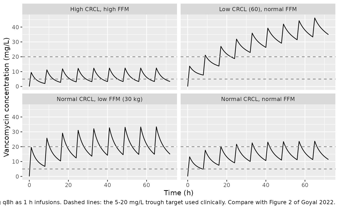
Figure 2 of the paper shows individual fits for patients with low, normal and high creatinine clearance and fat-free mass. The individual dosing histories are not published, so the figure below shows typical-value profiles for 1000 mg every 8 h (the median 3000 mg/day) as 1 h infusions, over the covariate combinations Figure 2 illustrates.
strata <- tibble::tribble(
  ~label,                          ~CRCL, ~FFM,
  "Normal CRCL, low FFM (30 kg)",   175,   30,
  "High CRCL, high FFM",            350,   60,
  "Normal CRCL, normal FFM",        175,   45,
  "Low CRCL (60), normal FFM",       60,   45
)
obs_times <- seq(0, 72, by = 0.25)
make_profile <- function(i) {
  doses <- data.frame(
    time = seq(0, 64, by = 8), evid = 1, amt = 1000, dur = 1,
    cmt = "central"
  )
  obs <- data.frame(time = obs_times, evid = 0, amt = 0, dur = 0, cmt = "central")
  dplyr::bind_rows(doses, obs) |>
    dplyr::arrange(time, dplyr::desc(evid)) |>
    dplyr::mutate(
      id = i, CRCL = strata$CRCL[i], FFM = strata$FFM[i],
      label = strata$label[i]
    )
}
prof_ev <- dplyr::bind_rows(lapply(seq_len(nrow(strata)), make_profile))
prof <- rxode2::rxSolve(mod_typ, prof_ev, keep = "label", returnType = "data.frame")
#> ℹ omega/sigma items treated as zero: 'etalcl'
#> Warning: multi-subject simulation without without 'omega'

ggplot(prof, aes(time, Cc)) +
  geom_line() +
  geom_hline(yintercept = c(5, 20), linetype = "dashed", colour = "grey50") +
  facet_wrap(~label) +
  labs(
    x = "Time (h)", y = "Vancomycin concentration (mg/L)",
    caption = paste(
      "Typical-value profiles, 1000 mg q8h as 1 h infusions.",
      "Dashed lines: the 5-20 mg/L trough target used clinically.",
      "Compare with Figure 2 of Goyal 2022."
    )
  )
Virtual cohort
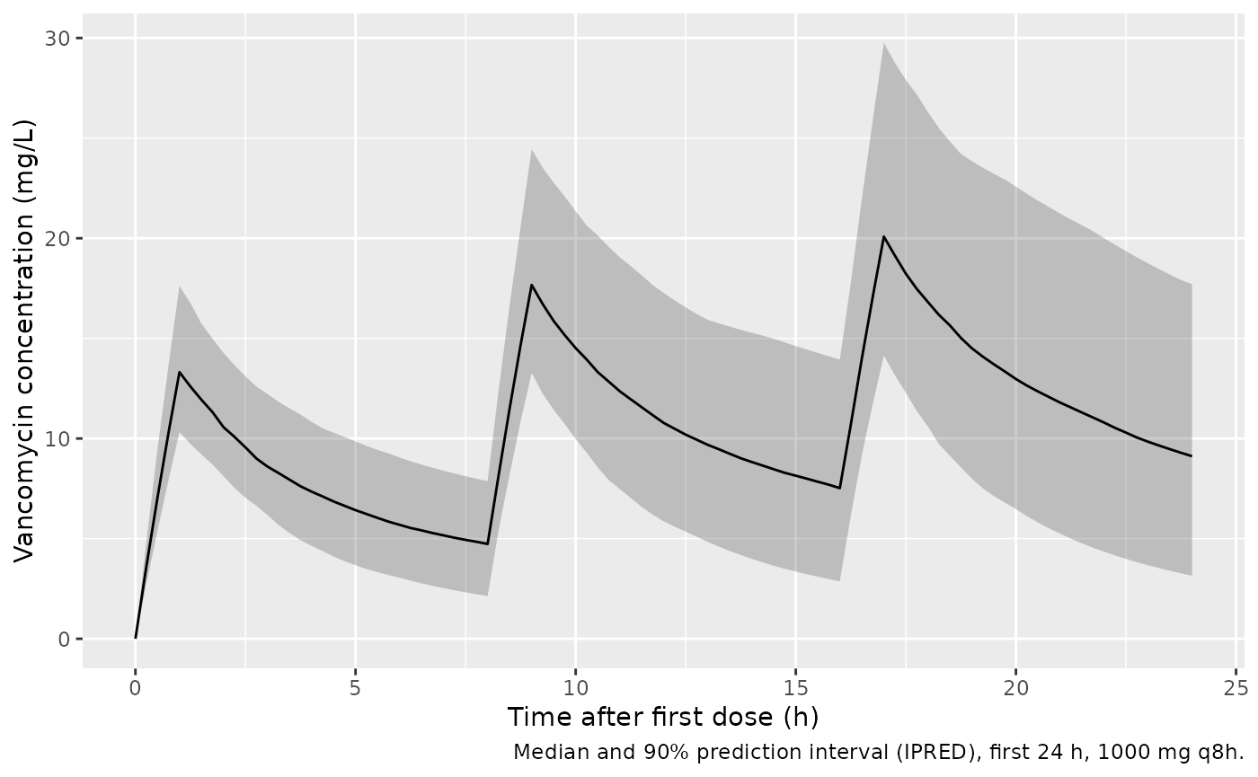
The individual patient data are not public. The virtual cohort draws
fat-free mass and creatinine clearance independently from log-normal
distributions centred on the Table 1 medians (45 kg and 176 mL/min) and
truncated to the Table 1 ranges. All subjects receive 1000 mg every 8 h
as 1 h infusions. Two event tables share the same subjects: one starting
from the first dose (for the paper’s AUC0-24), and one at steady state
(ss = 1 on the first record).
# set.seed() seeds R's RNG for the covariate draws. rxode2's own RNG (the eta
# and residual draws) is partitioned per solver thread, so the cohort differs
# across machines; every assertion below is written to hold for any cohort.
set.seed(20220606)
n_sub <- 200L
cov <- tibble::tibble(
  id = seq_len(n_sub),
  FFM = pmin(pmax(exp(rnorm(n_sub, log(45), 0.17)), 30), 60),
  CRCL = pmin(pmax(exp(rnorm(n_sub, log(176), 0.4)), 43), 389),
  treatment = "1000 mg q8h"
)
dose_times <- c(0, 8, 16)
obs_grid <- seq(0, 24, by = 0.25)
events <- dplyr::bind_rows(
  tidyr::crossing(cov, time = dose_times) |>
    dplyr::mutate(evid = 1L, amt = 1000, dur = 1, cmt = "central"),
  tidyr::crossing(cov, time = obs_grid) |>
    dplyr::mutate(evid = 0L, amt = 0, dur = 0, cmt = "central")
) |>
  dplyr::arrange(id, time, dplyr::desc(evid))
stopifnot(!anyDuplicated(unique(events[, c("id", "time", "evid")])))

# Steady state: the first dose record carries ss = 1, so the 0-24 h window is a
# steady-state dosing day.
events_ss <- events |>
  dplyr::mutate(
    ss = dplyr::if_else(evid == 1L & time == 0, 1L, 0L),
    ii = dplyr::if_else(evid == 1L & time == 0, 8, 0)
  )
Simulation
sim <- rxode2::rxSolve(
  mod, events = events, keep = c("treatment", "CRCL", "FFM"),
  returnType = "data.frame"
)
#> ℹ parameter labels from comments will be replaced by 'label()'
# Same seed for the steady-state solve. The eta draws need not match the first
# solve: the steady-state checks below compare each subject with its own CL.
rxode2::rxSetSeed(20220606)
sim_ss <- rxode2::rxSolve(
  mod, events = events_ss, keep = c("treatment", "CRCL", "FFM"),
  returnType = "data.frame", maxsteps = 1e6, rtol = 1e-10, atol = 1e-12,
  ssRtol = 1e-10, ssAtol = 1e-12
)
sim |>
  dplyr::filter(time <= 24) |>
  dplyr::group_by(time) |>
  dplyr::summarise(
    Q05 = quantile(Cc, 0.05), Q50 = median(Cc), Q95 = quantile(Cc, 0.95),
    .groups = "drop"
  ) |>
  ggplot(aes(time, Q50)) +
  geom_ribbon(aes(ymin = Q05, ymax = Q95), alpha = 0.25) +
  geom_line() +
  labs(
    x = "Time after first dose (h)", y = "Vancomycin concentration (mg/L)",
    caption = "Median and 90% prediction interval (IPRED), first 24 h, 1000 mg q8h."
  )
PKNCA validation
AUC over the first 24 h (the paper’s AUC0-24) and over a steady-state dosing day.
run_nca <- function(sim_df) {
  conc <- sim_df |>
    dplyr::filter(!is.na(Cc)) |>
    dplyr::select(id, time, Cc, treatment)
  dose_df <- events |>
    dplyr::filter(evid == 1) |>
    dplyr::select(id, time, amt, treatment)
  conc_obj <- PKNCA::PKNCAconc(conc, Cc ~ time | treatment + id)
  dose_obj <- PKNCA::PKNCAdose(
    dose_df, amt ~ time | treatment + id,
    route = "intravascular", duration = 1
  )
  intervals <- data.frame(start = 0, end = 24, auclast = TRUE, cmax = TRUE, cmin = TRUE)
  as.data.frame(PKNCA::pk.nca(PKNCA::PKNCAdata(conc_obj, dose_obj, intervals = intervals)))
}
nca_day1 <- run_nca(sim)
nca_ss <- run_nca(sim_ss)
auc_day1 <- nca_day1 |> dplyr::filter(PPTESTCD == "auclast")
auc_ss <- nca_ss |> dplyr::filter(PPTESTCD == "auclast")
stopifnot(nrow(auc_day1) == n_sub, nrow(auc_ss) == n_sub)
Steady-state mass balance
At steady state the AUC over one day equals the daily dose divided by each subject’s clearance. Both sides use the same simulated parameters, so the only difference is trapezoidal error on the 0.25 h grid.
cl_by_id <- sim_ss |> dplyr::distinct(id, cl)
ss_chk <- auc_ss |>
  dplyr::inner_join(cl_by_id, by = "id") |>
  dplyr::mutate(expected = 3000 / cl, pct_diff = 100 * (PPORRES / expected - 1))
stopifnot(nrow(ss_chk) == n_sub)
summary(ss_chk$pct_diff)
#>       Min.    1st Qu.     Median       Mean    3rd Qu.       Max.
#> -0.0962543 -0.0094055 -0.0055305 -0.0087260 -0.0031763 -0.0007461
# Measured max |difference| about 0.1% on the 0.25 h grid. A wrong dose, unit
# or ss handling moves this by tens of percent.
stopifnot(max(abs(ss_chk$pct_diff)) < 0.5)
Comparison against the published exposure
The paper reports a geometric mean (IQR) AUC0-24 of 223 (170-273) ugh/mL for the 34 patients simulated on their own dosing histories, and a median (IQR) individual-predicted trough of 10.1 (7.0-14.5) mg/L across patients and occasions. Neither the regimens nor the AUC window are published beyond that, so the comparison below (1000 mg q8h, first 24 h; troughs at steady state) is a plausibility check, not a reproduction. The paper’s method section says only that AUC0-24 was computed by NCA on the simulated profiles. The first-day window is the reading that matches: a steady-state dosing day gives a geometric mean far above 223 ugh/mL (shown below), and 223 ugh/mL is also well below the typical steady-state value of 3000 / 7.64 = 393 ugh/mL.
gm <- function(x) exp(mean(log(x)))
troughs_ss <- sim_ss |> dplyr::filter(time == 24) |> dplyr::pull(Cc)
simulated <- tibble::tibble(
  treatment = "1000 mg q8h",
  auclast = gm(auc_day1$PPORRES)
)
reference <- tibble::tibble(treatment = "1000 mg q8h", auclast = 223)
cmp <- nlmixr2lib::ncaComparisonTable(
  simulated = simulated, reference = reference, by = "treatment",
  units = c(auclast = "ug*h/mL"), tolerance_pct = 20
)
knitr::kable(
  cmp,
  caption = "Geometric mean AUC0-24 (first 24 h): simulated cohort vs Goyal 2022 Results. * differs by >20%."
)| NCA parameter | treatment | Reference | Simulated | % diff |
|---|---|---|---|---|
| AUClast (ug*h/mL) | 1000 mg q8h | 223 | 247 | +10.9% |
gm_day1 <- gm(auc_day1$PPORRES)
gm_ss <- gm(auc_ss$PPORRES)
# Centre-of-cohort check. The assumed regimen, not sampling noise, dominates
# the difference (the geometric mean of 200 subjects has an SE near 2%). The
# first-day reading sits about 10% above 223; a steady-state reading sits
# about 80% above it, which is why the paper's AUC0-24 is read as the first
# 24 h. A 2-fold error in CL or Vc pushes the first-day value outside 30%.
stopifnot(
  abs(gm_day1 / 223 - 1) < 0.3,
  gm_ss / 223 - 1 > 0.4
)

cat(sprintf("Geometric mean AUC0-24: first day %.0f, steady-state day %.0f ug*h/mL\n", gm_day1, gm_ss))
#> Geometric mean AUC0-24: first day 247, steady-state day 399 ug*h/mL

knitr::kable(
  tibble::tibble(
    Quantity = c("AUC0-24 (first day), ug*h/mL", "AUC over a steady-state day, ug*h/mL", "Trough at steady state, mg/L"),
    `Simulated median (IQR)` = c(
      sprintf("%.0f (%.0f-%.0f)", median(auc_day1$PPORRES), quantile(auc_day1$PPORRES, 0.25), quantile(auc_day1$PPORRES, 0.75)),
      sprintf("%.0f (%.0f-%.0f)", median(auc_ss$PPORRES), quantile(auc_ss$PPORRES, 0.25), quantile(auc_ss$PPORRES, 0.75)),
      sprintf("%.1f (%.1f-%.1f)", median(troughs_ss), quantile(troughs_ss, 0.25), quantile(troughs_ss, 0.75))
    ),
    `Goyal 2022` = c("geometric mean 223 (IQR 170-273)", "not reported", "median 10.1 (IQR 7.0-14.5), all occasions")
  ),
  caption = "Simulated exposure summaries and the values the paper reports."
)| Quantity | Simulated median (IQR) | Goyal 2022 |
|---|---|---|
| AUC0-24 (first day), ug*h/mL | 251 (209-298) | geometric mean 223 (IQR 170-273) |
| AUC over a steady-state day, ug*h/mL | 406 (292-535) | not reported |
| Trough at steady state, mg/L | 12.3 (7.5-17.1) | median 10.1 (IQR 7.0-14.5), all occasions |
Assumptions and deviations
- Dosing regimen and infusion duration. The paper reports only the median (IQR) daily dose, 3000 mg (2000-4000 mg), and no infusion duration. The simulations use 1000 mg every 8 h as 1 h infusions. The published AUC0-24 and trough summaries came from each patient’s own dosing history, so the comparison table is a plausibility check rather than a reproduction.
- AUC0-24 window. The paper does not state which 24 h its AUC0-24 covers. The maintainers read it as the first 24 h after the first dose: that reading lands within about 10% of the published geometric mean, while a steady-state day lands about 80% above it. The simulated steady-state trough (median about 12 mg/L) is close to the paper’s median individual-predicted trough of 10.1 mg/L, which pools all dosing occasions, including those before steady state.
- Covariate distributions. Fat-free mass and creatinine clearance are drawn independently from log-normal distributions on the Table 1 medians and truncated at the Table 1 ranges; the spreads (log-SD 0.17 and 0.4) were chosen by the maintainers to roughly match those ranges. In real patients the two are correlated through the Cockcroft-Gault weight term.
-
IIV scale. Table 2 reports IIV on CL as 31.9 CV%.
The Pumas code declares
etaCL ~ Normal(0, OmegaCL), so the estimated quantity is a standard deviation; the variance used here islog(1 + 0.319^2) = 0.0969. Reading the 31.9% as the SD itself would give0.319^2 = 0.102, a 5% difference in variance that does not materially change any simulation. -
Truncated residual error. The model was fitted with
a normal residual truncated below at the 5 mg/L LLOQ (Beal’s M2 method;
Supplementary Code S1
truncated(Normal(cp, abs(cp) * sigma_prop), 4.99999, Inf)). The truncation is a fitting device for the below-LLOQ exclusions and is not reproduced in simulation:Cc ~ prop(propSd)simulates the untruncated proportional error. To refit with comparable handling, censor or exclude the below-LLOQ records in the data. -
Fixed parameters. Q, Vp and the
creatinine-clearance exponent are encoded as
fixed()because the authors held them at the non-pregnant base-model values. Q uses 9.064 L/h from the published code; Table 2 rounds it to 9.06. - Non-pregnant base model not packaged. Supplementary Table S1 is the starting model, taken from the literature and modified by the authors, and was used only for the pregnant/non-pregnant AUC comparison. Its parameters are shown above for reference; it is not packaged as a separate model.
- Pregnancy-related body composition. Fat-free mass in the source comes from the Janmahasatian formula on total body weight, which in pregnancy includes the fetus, placenta and amniotic fluid. The paper makes no adjustment, and neither does this model; users should compute FFM the same way.
- No erratum or correction notice for the paper was found in Europe PMC as of 2026-10-01.