Varenicline and cigarette craving (Ravva 2015)
Source:vignettes/articles/Ravva_2015_varenicline.Rmd
Ravva_2015_varenicline.RmdModel and source
mod <- readModelDb("Ravva_2015_varenicline")
ui  <- rxode2::rxode(mod)
#> ℹ parameter labels from comments will be replaced by 'label()'- Citation: Ravva P, Gastonguay MR, Faessel HM, Lee TC, Niaura R. Pharmacokinetic-pharmacodynamic modeling of the effect of varenicline on nicotine craving in adult smokers. Nicotine Tob Res. 2015;17(1):106-113. doi:10.1093/ntr/ntu154
- Article: https://doi.org/10.1093/ntr/ntu154 (PMC4832970)
- Supplement: Supplementary Table S1 and Figures S1-S5, deposited with the PMC record. Every parameter of the model lives in Table S1 – the main text prints none.
Structure
Ravva 2015 Figure 1 draws two kinetic systems side by side and one effect equation:
DRUG DOSE -> DEPOT --ka--> CENTRAL (C_DRUG) <--Q/V2, Q/V3--> PERIPHERAL,  CL/V2 out
PBO "DOSE" -> DEPOT --kon--> "C_PBO" --koff--> out

EFFECT = E0 + PSLP * C_PBO + DSLP * C_DRUG
Three points about that structure govern the whole encoding.
The PK layer was not estimated here. Ravva 2015
Methods: “The final PK model and population parameters previously
obtained in a varenicline pooled analysis were used as prior information
in a maximum a posteriori (MAP) Bayesian analysis (POSTHOC option) of
the new PK data from this study.” That pooled analysis is reference 30,
Ravva 2009, which is packaged here as
modellib("Ravva_2009_varenicline"). Every PK fixed effect
and the whole PK IIV block are transcribed from that packaged sibling
model and wrapped in fixed(), because in the Ravva 2015
analysis they are prior constants.
The placebo system is hypothetical. Methods: “The
time-varying behavior of the placebo response was modeled as a separate
hypothetical kinetic system with a ‘dummy’ unit dose introduced at times
of placebo or varenicline dosing.” A dose of exactly 1 (dimensionless)
enters depot_placebo; central_placebo holds
the paper’s C_PBO. With a unit bolus this gives
C_PBO(t) = kon / (koff - kon) * (exp(-kon * t) - exp(-koff * t))which is what a NONMEM ADVAN5 general-linear system returns for that chain. The unit-dose convention is load-bearing; it is checked against the paper’s own simulations below.
The effect model lives on the logit scale. Table S1
footnote b: “Parameters are presented in the logit scale as data were
modeled using logistic transformation to constrain between 0 and 100.”
So the packaged model computes
smokingurges <- expit(EFFECT, 0, 100) and carries a
logitNorm(addSd, 0, 100) residual, which puts the additive
residual SD on the same logit scale the three effect parameters live
on.
Population
Forty adult smokers (21 male, 19 female), mean age 36 years (range 18-63), mean body weight 77 kg for males (range 59-95) and 72 kg for females (range 58-90), 39 of 40 (97.5%) White, enrolled at a single United States centre. Inclusion required at least 20 cigarettes/day, or 11-19 cigarettes/day with the first cigarette within 30 minutes of waking, and no current intent to quit. Subjects smoked about 21 cigarettes/day (range 16-40), had smoked since age 17 (range 12-31), and scored 5.6 (SE 0.31) of 10 on the Fagerstrom Test for Nicotine Dependence; 7 of 40 reported prior bupropion quit attempts.
The design was a randomized, double-blind, placebo-controlled, two-period crossover with a 7-day washout, comparing a single 2 mg oral dose (2 x 1 mg tablets) of varenicline against placebo. Subjects were abstinent from smoking and food overnight, confirmed with exhaled CO below 15 ppm. Only the abstinence window from time 0 to 4 h postdose – before the scripted cue-reactivity session – was analysed, to avoid confounding by cue exposure. The dataset comprised 305 varenicline concentrations, 387 placebo-period craving responses and 390 varenicline-period craving responses. (Ravva 2015 Methods “Study Design” / “Study Procedures”; Results “Subject Disposition and Smoking History”.)
str(mod()$population)
#> List of 14
#>  $ species       : chr "human"
#>  $ n_subjects    : int 40
#>  $ n_studies     : int 1
#>  $ age_range     : chr "18-63 years"
#>  $ age_mean      : chr "36 years"
#>  $ weight_range  : chr "59-95 kg (males); 58-90 kg (females)"
#>  $ weight_mean   : chr "77 kg (males); 72 kg (females)"
#>  $ sex_female_pct: num 47.5
#>  $ race_ethnicity: Named num [1:2] 97.5 2.5
#>   ..- attr(*, "names")= chr [1:2] "White" "Other"
#>  $ disease_state : chr "Otherwise healthy adult smokers aged 18-65 not currently intending to quit, smoking at least 20 cigarettes/day,"| __truncated__
#>  $ dose_range    : chr "Single 2 mg oral dose (2 x 1 mg tablets) of varenicline versus placebo"
#>  $ regions       : chr "Single center, United States (Center for Behavioral Medicine, The Miriam Hospital)"
#>  $ samples       : chr "305 varenicline plasma concentrations, 387 placebo-period craving responses and 390 varenicline-period craving "| __truncated__
#>  $ notes         : chr "Randomized, double-blind, placebo-controlled, two-period crossover with a 7-day washout (Ravva 2015 Methods, 'S"| __truncated__
Source trace
Every ini() value carries an in-file comment naming its
source. They are collected here for review.
| Equation / parameter | Value | Source location |
|---|---|---|
| 2-compartment PK ODEs, first-order absorption, absorption lag | n/a | Ravva 2015 Figure 1 (structure) with parameters from Ravva 2009
Table 4, via Ravva_2009_varenicline.R
|
lka, lcl, lvc,
lvp, lq, ltlag
|
log(1.69), log(10.4),
log(337), log(78.1), log(2.08),
log(0.43)
|
Ravva 2009 Table 4 final model; fixed() because Ravva
2015 used them as MAP-Bayesian priors, not estimates |
e_crcl_cl, e_black_cl,
e_other_cl
|
0.54, 1.16, 1.11 | Ravva 2009 Table 4 (q_CRCL, q_Black, q_Other on CL/F) |
e_wt_vc, e_age_vc,
e_black_vc, e_other_vc
|
0.77, 0.13, 0.92, 0.71 | Ravva 2009 Table 4 (on V2/F) |
e_wt_vp, e_wt_q
|
1, 0.75 | Ravva 2009 Table 4, reported as Fixed |
PK IIV block on etalka, etalcl,
etalvc
|
0.49 / -0.009, 0.061 / 0.24, 0.006, 0.25 | Ravva 2009 Table 4 interindividual-variance BLOCK |
| Placebo kinetic system, dummy unit dose at each dosing time | n/a | Ravva 2015 Methods, “Pharmacokinetic and Pharmacodynamic Analyses”; Figure 1 right-hand box |
lkon_placebo |
fixed(log(0.0112)) |
Ravva 2015 Supplementary Table S1: k_on = 0.0112 /h (%RSE 142); fixed per Table S1 footnote a |
lkoff_placebo |
fixed(log(0.130)) |
Ravva 2015 Supplementary Table S1: k_off = 0.130 /h (%RSE 65.4); fixed per Table S1 footnote a |
etalkon_placebo, etalkoff_placebo
|
fixed(0.97987), fixed(0.88216)
|
Table S1 %CV = 129 and 119; omega^2 = log(1 + CV^2) |
EFFECT = E0 + PSLP * C_PBO + DSLP * C_DRUG |
n/a | Ravva 2015 Figure 1 equation box; Methods paragraph on the linear PD model |
logite0 |
0.991 | Supplementary Table S1: E0 = 0.991 (%RSE 29.6), logit scale per footnote b |
slope_placebo (PSLP) |
-3.32 | Supplementary Table S1: PSLP = -3.32 (%RSE 50.6) |
slope_drug (DSLP) |
-0.192 | Supplementary Table S1: DSLP = -0.192 (%RSE 33.5) |
etalogite0, etaslope_placebo,
etaslope_drug
|
3.2041, 16.1604, 0.157609 | Table S1 IIV SDs 1.79, 4.02, 0.397, squared; additive per Methods (“Inter-individual and residual random effects were characterized by an additive error model”) |
addSd |
1.06 | Supplementary Table S1 residual-error row: sigma_(3,3) add,PD SD = 1.06 (%RSE 17.0), additive on the logit scale |
smokingurges <- expit(EFFECT, 0, 100) |
n/a | Supplementary Table S1 footnote b (logistic transformation constraining 0-100) |
Validation 1: the paper’s own forward simulations
Ravva 2015 Figure 4 and Supplementary Figure S3 are Monte Carlo
forward simulations “based on the final model and parameter estimates”.
They are the strongest available check on the encoding, because they
exercise the placebo system over 14 days of repeated dosing where
accumulation dominates the response. The published black line is a
median over 500 replicate trials of 40 subjects including parameter
uncertainty; the packaged model is compared against it as a
typical-value (zeroRe) solve.
mod_typ <- rxode2::zeroRe(mod)
#> ℹ parameter labels from comments will be replaced by 'label()'

# Reference covariates of the Ravva 2009 PK layer.
ref_cov <- data.frame(CRCL = 100, WT = 70, AGE = 45, RACE_BLACK = 0, RACE_OTHER = 0)

# Every dosing time gets BOTH the varenicline dose and the dimensionless
# placebo dummy dose of 1 (Ravva 2015 Methods).
dose_rows <- function(times, amt) {
  dplyr::bind_rows(
    data.frame(time = times, amt = amt, cmt = "depot",         evid = 1L),
    data.frame(time = times, amt = 1,   cmt = "depot_placebo", evid = 1L)
  )
}

obs_rows <- data.frame(time = seq(0, 15 * 24, by = 0.25), amt = 0,
                       cmt = "central", evid = 0L)

solve_regimen <- function(doses, params = NULL) {
  ev <- dplyr::bind_rows(doses, obs_rows) |>
    dplyr::arrange(time, dplyr::desc(evid)) |>
    dplyr::mutate(id = 1L)
  ev <- dplyr::bind_cols(ev, ref_cov[rep(1, nrow(ev)), ])
  if (is.null(params)) {
    rxode2::rxSolve(mod_typ, ev, omega = NA, sigma = NA, returnType = "data.frame")
  } else {
    rxode2::rxSolve(mod_typ, ev, params = params, omega = NA, sigma = NA,
                    returnType = "data.frame")
  }
}

# Figure 4: 0.5 mg q.d. for 3 days, 0.5 mg b.i.d. for 4 days, then 1 mg b.i.d.
titrated_doses <- dplyr::bind_rows(
  dose_rows(c(0, 24, 48), 0.5),
  dose_rows(as.vector(outer(c(0, 12), 72 + 24 * (0:3), "+")), 0.5),
  dose_rows(as.vector(outer(c(0, 12), 168 + 24 * (0:7), "+")), 1)
)
sim_titrated <- solve_regimen(titrated_doses)
# Figure S3: non-titrated 1 mg q.d. and 1 mg b.i.d.
sim_qd  <- solve_regimen(dose_rows(24 * (0:14), 1))
sim_bid <- solve_regimen(dose_rows(as.vector(outer(c(0, 12), 24 * (0:14), "+")), 1))
day_panels <- c(1, 2, 3, 4, 7, 14)

# Each published panel shows one day on a 0-24 h axis, so the window is
# closed at BOTH ends: t = 24 h appears as hour 24 of day 1 and as hour 0 of
# day 2, exactly as it does in the figure.
panel_frame <- function(sim, arm) {
  do.call(rbind, lapply(day_panels, function(d) {
    lo <- (d - 1) * 24
    s <- sim[sim$time >= lo & sim$time <= lo + 24, ]
    data.frame(arm = arm, day = d, hour = s$time - lo,
               smokingurges = s$smokingurges)
  }))
}

chronic <- dplyr::bind_rows(
  panel_frame(sim_titrated, "Titrated (Figure 4)"),
  panel_frame(sim_qd,  "1 mg q.d. (Figure S3)"),
  panel_frame(sim_bid, "1 mg b.i.d. (Figure S3)")
)

ggplot(chronic, aes(hour, smokingurges, colour = arm)) +
  geom_line() +
  facet_wrap(~ paste("Day", day), ncol = 3) +
  scale_x_continuous(breaks = seq(0, 24, by = 4)) +
  coord_cartesian(ylim = c(0, 100)) +
  labs(x = "Time (h)", y = "Craving score (Smoking Urges Scale mean 1-5)",
       colour = NULL,
       title = "Typical-value craving response under chronic varenicline",
       caption = "Replicates Figure 4 (titrated) and Supplementary Figure S3 of Ravva 2015.") +
  theme(legend.position = "bottom")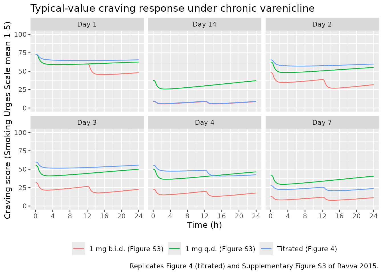
Quantitative comparison against the published panels
Thirty points were read off the three published panel sets. Digitisation from a printed figure carries roughly plus or minus 2 craving points of reading error, which sets the scale of what the comparison can resolve.
published_panels <- tibble::tribble(
  ~arm,                    ~day, ~hour, ~published,
  "Titrated (Figure 4)",      1,   0.5,      71.5,
  "Titrated (Figure 4)",      1,  24.0,      64.5,
  "Titrated (Figure 4)",      2,   8.0,      55.5,
  "Titrated (Figure 4)",      2,  24.0,      58.5,
  "Titrated (Figure 4)",      3,   8.0,      50.5,
  "Titrated (Figure 4)",      3,  24.0,      54.5,
  "Titrated (Figure 4)",      4,   8.0,      46.5,
  "Titrated (Figure 4)",      4,  24.0,      41.5,
  "Titrated (Figure 4)",      7,   8.0,      24.0,
  "Titrated (Figure 4)",      7,  24.0,      26.0,
  "Titrated (Figure 4)",     14,   8.0,      10.5,
  "Titrated (Figure 4)",     14,  24.0,      13.0,
  "1 mg q.d. (Figure S3)",    2,   4.0,      48.5,
  "1 mg q.d. (Figure S3)",    2,  24.0,      55.0,
  "1 mg q.d. (Figure S3)",    4,   8.0,      38.0,
  "1 mg q.d. (Figure S3)",    4,  24.0,      47.0,
  "1 mg q.d. (Figure S3)",    7,   8.0,      32.5,
  "1 mg q.d. (Figure S3)",    7,  24.0,      42.0,
  "1 mg q.d. (Figure S3)",   14,   8.0,      30.0,
  "1 mg q.d. (Figure S3)",   14,  24.0,      39.0,
  "1 mg b.i.d. (Figure S3)",  1,   8.0,      59.0,
  "1 mg b.i.d. (Figure S3)",  1,  24.0,      48.0,
  "1 mg b.i.d. (Figure S3)",  2,   8.0,      36.5,
  "1 mg b.i.d. (Figure S3)",  2,  24.0,      33.0,
  "1 mg b.i.d. (Figure S3)",  4,   8.0,      19.5,
  "1 mg b.i.d. (Figure S3)",  4,  24.0,      21.0,
  "1 mg b.i.d. (Figure S3)",  7,   8.0,      13.0,
  "1 mg b.i.d. (Figure S3)",  7,  24.0,      16.0,
  "1 mg b.i.d. (Figure S3)", 14,   8.0,      11.0,
  "1 mg b.i.d. (Figure S3)", 14,  24.0,      13.5
)

chk <- published_panels |>
  dplyr::left_join(
    chronic |> dplyr::mutate(hour = round(hour, 2)),
    by = c("arm", "day", "hour")
  ) |>
  dplyr::mutate(diff = smokingurges - published)

chk |>
  dplyr::mutate(dplyr::across(c(smokingurges, diff), function(x) round(x, 1))) |>
  dplyr::rename("Arm" = arm, "Day" = day, "Time (h)" = hour,
                "Published" = published, "Model" = smokingurges,
                "Model - published" = diff) |>
  knitr::kable(caption = paste(
    "Typical-value craving response versus values read off Figure 4 and",
    "Supplementary Figure S3 of Ravva 2015."
))| Arm | Day | Time (h) | Published | Model | Model - published |
|---|---|---|---|---|---|
| Titrated (Figure 4) | 1 | 0.5 | 71.5 | 71.9 | 0.4 |
| Titrated (Figure 4) | 1 | 24.0 | 64.5 | 65.4 | 0.9 |
| Titrated (Figure 4) | 2 | 8.0 | 55.5 | 57.0 | 1.5 |
| Titrated (Figure 4) | 2 | 24.0 | 58.5 | 59.7 | 1.2 |
| Titrated (Figure 4) | 3 | 8.0 | 50.5 | 51.7 | 1.2 |
| Titrated (Figure 4) | 3 | 24.0 | 54.5 | 55.5 | 1.0 |
| Titrated (Figure 4) | 4 | 8.0 | 46.5 | 47.8 | 1.3 |
| Titrated (Figure 4) | 4 | 24.0 | 41.5 | 42.5 | 1.0 |
| Titrated (Figure 4) | 7 | 8.0 | 24.0 | 23.8 | -0.2 |
| Titrated (Figure 4) | 7 | 24.0 | 26.0 | 23.9 | -2.1 |
| Titrated (Figure 4) | 14 | 8.0 | 10.5 | 7.6 | -2.9 |
| Titrated (Figure 4) | 14 | 24.0 | 13.0 | 9.0 | -4.0 |
| 1 mg q.d. (Figure S3) | 2 | 4.0 | 48.5 | 48.1 | -0.4 |
| 1 mg q.d. (Figure S3) | 2 | 24.0 | 55.0 | 55.1 | 0.1 |
| 1 mg q.d. (Figure S3) | 4 | 8.0 | 38.0 | 38.1 | 0.1 |
| 1 mg q.d. (Figure S3) | 4 | 24.0 | 47.0 | 46.4 | -0.6 |
| 1 mg q.d. (Figure S3) | 7 | 8.0 | 32.5 | 31.5 | -1.0 |
| 1 mg q.d. (Figure S3) | 7 | 24.0 | 42.0 | 40.6 | -1.4 |
| 1 mg q.d. (Figure S3) | 14 | 8.0 | 30.0 | 27.8 | -2.2 |
| 1 mg q.d. (Figure S3) | 14 | 24.0 | 39.0 | 37.1 | -1.9 |
| 1 mg b.i.d. (Figure S3) | 1 | 8.0 | 59.0 | 59.2 | 0.2 |
| 1 mg b.i.d. (Figure S3) | 1 | 24.0 | 48.0 | 48.0 | 0.0 |
| 1 mg b.i.d. (Figure S3) | 2 | 8.0 | 36.5 | 36.5 | 0.0 |
| 1 mg b.i.d. (Figure S3) | 2 | 24.0 | 33.0 | 31.7 | -1.3 |
| 1 mg b.i.d. (Figure S3) | 4 | 8.0 | 19.5 | 17.6 | -1.9 |
| 1 mg b.i.d. (Figure S3) | 4 | 24.0 | 21.0 | 17.8 | -3.2 |
| 1 mg b.i.d. (Figure S3) | 7 | 8.0 | 13.0 | 10.1 | -2.9 |
| 1 mg b.i.d. (Figure S3) | 7 | 24.0 | 16.0 | 11.4 | -4.6 |
| 1 mg b.i.d. (Figure S3) | 14 | 8.0 | 11.0 | 7.1 | -3.9 |
| 1 mg b.i.d. (Figure S3) | 14 | 24.0 | 13.5 | 8.6 | -4.9 |
summary_stats <- c(
  median = median(abs(chk$diff)),
  q90    = unname(quantile(abs(chk$diff), 0.9)),
  max    = max(abs(chk$diff))
)
round(summary_stats, 2)
#> median    q90    max
#>   1.25   3.87   4.90

# This solve is deterministic (zeroRe, no random draws), so the only slack the
# bounds need is figure-digitisation error. Observed on authoring:
# median 1.25, q90 3.87, max 4.90 craving points. A mis-transcribed slope,
# rate constant or dose unit moves the whole set by tens of points and blows
# all three instantly.
stopifnot(
  summary_stats[["median"]] < 3,
  summary_stats[["q90"]]    < 6,
  summary_stats[["max"]]    < 8
)
The residual pattern is informative rather than worrying: the model sits within a point or two of the published line everywhere except the late, low-response panels (days 7 and 14 of the b.i.d. arms), where it runs 3-5 points low. That is the expected direction. The published line is a median over subjects and the logit back-transform is convex near the bottom of the scale, so a cohort median sits above the typical-value curve exactly where the response is small.
The C_PBO amplitude convention
A unit dummy dose fixes the amplitude of C_PBO, and
therefore the meaning of slope_placebo. An alternative
koff-normalised convention is shape
identical and differs only by the factor
koff / kon = 11.6, so no time-course argument can separate
the two – and the parameter names cannot either, because with
kon < koff the rise of the Bateman curve is governed by
the larger constant under both readings. The paper’s own forward
simulations settle it.
alt_mult <- 0.130 / 0.0112   # koff / kon

alt <- solve_regimen(titrated_doses,
                     params = c(slope_placebo = -3.32 * alt_mult))

at_time <- function(sim, day, hour) {
  sim$smokingurges[which.min(abs(sim$time - ((day - 1) * 24 + hour)))]
}

conv <- tibble::tibble(
  Convention = c("Unit dummy dose (packaged model)",
                 "koff-normalised alternative"),
  `Day 3, 8 h`  = c(at_time(sim_titrated, 3, 8),  at_time(alt, 3, 8)),
  `Day 7, 8 h`  = c(at_time(sim_titrated, 7, 8),  at_time(alt, 7, 8)),
  `Day 14, 8 h` = c(at_time(sim_titrated, 14, 8), at_time(alt, 14, 8))
) |>
  dplyr::mutate(dplyr::across(where(is.numeric), function(x) round(x, 1)))

knitr::kable(conv, caption = paste(
  "Figure 4 of Ravva 2015 reads about 50.5, 24.0 and 10.5 craving points at",
  "these three times. The koff-normalised convention is falsified."
))| Convention | Day 3, 8 h | Day 7, 8 h | Day 14, 8 h |
|---|---|---|---|
| Unit dummy dose (packaged model) | 51.7 | 23.8 | 7.6 |
| koff-normalised alternative | 0.3 | 0.0 | 0.0 |
stopifnot(at_time(alt, 3, 8) < 20) # published value is about 50.5Validation 2: the observed 4-hour profiles (Figure 2)
Figure 2 of Ravva 2015 shows the observed mean time-course of varenicline concentration and of craving over the 4-hour abstinence window, for both crossover periods. A 200-subject virtual cohort per arm is simulated with the full published random effects.
# rxSetSeed fixes rxode2's stream within an rxode2 version but not across
# versions or solver-thread counts, so every assertion below is written on a
# centre or a robust quantile, never on a cohort extreme.
rxode2::rxSetSeed(20150117)
set.seed(20150117)

n_arm <- 200

make_cohort <- function(n, id_offset = 0L) {
  sexf <- rep(c(0, 1), length.out = n)         # 21 M / 19 F in the trial
  tibble::tibble(
    id   = id_offset + seq_len(n),
    SEXF = sexf,
    WT   = ifelse(sexf == 0, rnorm(n, 77, 9), rnorm(n, 72, 8)),
    AGE  = pmin(pmax(rnorm(n, 36, 11), 18), 63),
    RACE_BLACK = 0,
    RACE_OTHER = 0
  ) |>
    # Serum creatinine is not reported; 0.9 mg/dL is assumed (see Assumptions).
    dplyr::mutate(
      WT   = pmin(pmax(WT, 58), 95),
      CRCL = (140 - AGE) * WT / (72 * 0.9) * ifelse(SEXF == 1, 0.85, 1)
    )
}

pd_times <- seq(0, 4, by = 0.5)                       # craving assessments
pk_times <- c(0, 0.5, 1, 1.5, 2, 2.5, 3, 3.5, 4, 5.25, 5.75, 6.25)  # blood draws
obs_times <- sort(unique(c(pd_times, pk_times)))

expand_arm <- function(cohort, dose, arm) {
  # The placebo arm still receives the dimensionless dummy dose; only the
  # varenicline arm additionally receives drug.
  dose_grid <- if (dose > 0) {
    data.frame(time = 0, amt = c(dose, 1),
               cmt = c("depot", "depot_placebo"), evid = 1L)
  } else {
    data.frame(time = 0, amt = 1, cmt = "depot_placebo", evid = 1L)
  }
  obs_grid <- data.frame(time = obs_times, amt = 0, cmt = "central", evid = 0L)

  dplyr::bind_rows(
    merge(cohort, dose_grid),
    merge(cohort, obs_grid)
  ) |>
    dplyr::mutate(arm = arm) |>
    dplyr::arrange(id, time, dplyr::desc(evid))
}

events <- dplyr::bind_rows(
  expand_arm(make_cohort(n_arm, id_offset = 0L),     2, "Varenicline 2 mg"),
  expand_arm(make_cohort(n_arm, id_offset = n_arm), 0, "Placebo")
)
stopifnot(!anyDuplicated(unique(events[, c("id", "time", "evid")])))
sim <- rxode2::rxSolve(mod, events = events, keep = c("arm", "WT", "AGE", "CRCL"),
                       returnType = "data.frame")
#> ℹ parameter labels from comments will be replaced by 'label()'
observed_fig2 <- tibble::tribble(
  ~arm,               ~time, ~obs_craving, ~obs_Cc,
  "Varenicline 2 mg",   0.0,         67.5,      NA,
  "Varenicline 2 mg",   0.5,         50.0,     1.6,
  "Varenicline 2 mg",   1.0,         42.5,     3.8,
  "Varenicline 2 mg",   1.5,         41.5,     5.6,
  "Varenicline 2 mg",   2.0,         37.5,     6.4,
  "Varenicline 2 mg",   2.5,         36.0,     7.0,
  "Varenicline 2 mg",   3.0,         34.0,     7.4,
  "Varenicline 2 mg",   3.5,         31.5,     7.3,
  "Varenicline 2 mg",   4.0,         30.0,    7.45,
  "Placebo",            0.0,         64.5,      NA,
  "Placebo",            0.5,         53.5,      NA,
  "Placebo",            1.0,         52.0,      NA,
  "Placebo",            1.5,         47.0,      NA,
  "Placebo",            2.0,         44.0,      NA,
  "Placebo",            2.5,         44.5,      NA,
  "Placebo",            3.0,         42.5,      NA,
  "Placebo",            3.5,         44.0,      NA,
  "Placebo",            4.0,         45.5,      NA
)

sim_mean <- sim |>
  dplyr::filter(time %in% pd_times) |>
  dplyr::group_by(arm, time) |>
  dplyr::summarise(craving = mean(smokingurges), .groups = "drop")

ggplot(sim_mean, aes(time, craving, colour = arm)) +
  geom_line() +
  geom_point(data = observed_fig2, aes(time, obs_craving, colour = arm),
             shape = 1, size = 2.5, inherit.aes = FALSE) +
  coord_cartesian(ylim = c(0, 100)) +
  labs(x = "Time postdose (h)",
       y = "Mean (1-5) craving score",
       colour = NULL,
       title = "Cohort-mean craving over the 4 h abstinence window",
       caption = paste("Lines: 200-subject simulation per arm. Open circles:",
                       "means read off Figure 2 of Ravva 2015.")) +
  theme(legend.position = "bottom")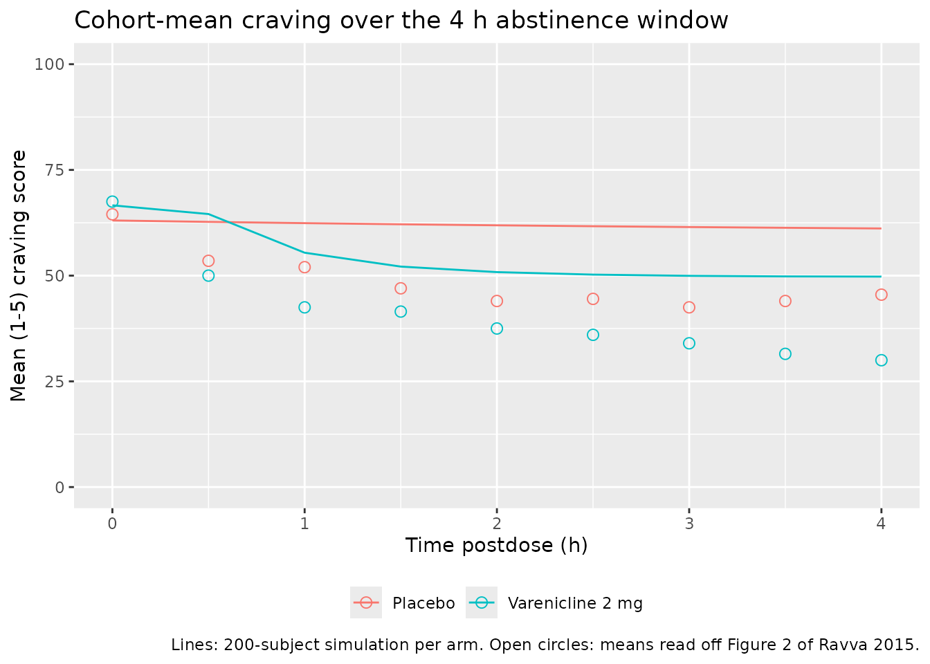
baseline <- sim_mean |> dplyr::filter(time == 0)

baseline |>
  dplyr::mutate(craving = round(craving, 1)) |>
  dplyr::rename("Arm" = arm, "Time (h)" = time, "Mean craving at baseline" = craving) |>
knitr::kable(caption = "Simulated baseline craving versus 64.5-67.5 read off Figure 2.")| Arm | Time (h) | Mean craving at baseline |
|---|---|---|
| Placebo | 0 | 65.3 |
| Varenicline 2 mg | 0 | 66.3 |
# The full-IIV cohort mean at t = 0 is well below the typical-value baseline of
# 100 * expit(0.991) = 72.9, because the additive eta on the logit-scale
# baseline (SD 1.79) is large and the back-transform is concave at that point.
# Published baselines are 67.5 (varenicline period) and 64.5 (placebo period).
stopifnot(all(baseline$craving > 50), all(baseline$craving < 80))
The simulated baselines land on the observed ones. The simulated placebo time-course, however, is nearly flat (about 3 craving points of decline over 4 h) where the observed placebo mean falls about 20 points, and the varenicline arm falls short by a similar margin. This is a real and expected limitation of a population forward simulation of this model, discussed under Assumptions below; it is not a transcription error, and the chronic-simulation check above is what pins the encoding.
PKNCA validation
The paper reports non-compartmental Cmax and Tmax derived directly from the observed concentrations after the single 2 mg dose, sampled predose and at 0.5, 1, 1.5, 2, 2.5, 3, 3.5, 4, 5.25, 5.75 and 6.25 h. The NCA below uses exactly that schedule so the comparison is like for like.
sim_nca <- sim |>
  dplyr::filter(arm == "Varenicline 2 mg", time %in% pk_times) |>
  dplyr::filter(!is.na(Cc)) |>
  dplyr::select(id, time, Cc, arm)

# Guarantee a time-zero record per subject (Cc = 0 predose, extravascular).
sim_nca <- dplyr::bind_rows(
  sim_nca,
  sim_nca |> dplyr::distinct(id, arm) |> dplyr::mutate(time = 0, Cc = 0)
) |>
  dplyr::distinct(id, arm, time, .keep_all = TRUE) |>
  dplyr::arrange(id, time)

dose_df <- events |>
  dplyr::filter(evid == 1, cmt == "depot", arm == "Varenicline 2 mg") |>
  dplyr::select(id, time, amt, arm)

conc_obj <- PKNCA::PKNCAconc(sim_nca, Cc ~ time | arm + id)
dose_obj <- PKNCA::PKNCAdose(dose_df, amt ~ time | arm + id)

intervals <- data.frame(start = 0, end = 6.25, cmax = TRUE, tmax = TRUE,
                        auclast = TRUE)

nca_res <- PKNCA::pk.nca(PKNCA::PKNCAdata(conc_obj, dose_obj, intervals = intervals))
# Ravva 2015 reports Cmax as a MEAN (SD) and Tmax as a MEDIAN (range), so the
# simulated side is pre-aggregated with the matching statistic rather than
# letting ncaComparisonTable() take a median of both.
sim_summary <- nca_res$result |>
  dplyr::filter(PPTESTCD %in% c("cmax", "tmax")) |>
  dplyr::group_by(arm, PPTESTCD) |>
  dplyr::summarise(mean_val = mean(PPORRES), med_val = median(PPORRES),
                   .groups = "drop") |>
  dplyr::mutate(PPORRES = ifelse(PPTESTCD == "cmax", mean_val, med_val)) |>
  dplyr::select(arm, PPTESTCD, PPORRES)

published_nca <- tibble::tribble(
  ~arm,               ~cmax, ~tmax,
  "Varenicline 2 mg",  8.27,  3.00
)

cmp <- nlmixr2lib::ncaComparisonTable(
  simulated     = sim_summary,
  reference     = published_nca,
  by            = "arm",
  units         = c(cmax = "ng/mL", tmax = "h"),
  tolerance_pct = 20
)

knitr::kable(cmp, caption = paste(
  "Simulated versus published NCA for the single 2 mg dose.",
  "* differs from the reference by more than 20%.",
  "Published Cmax is a mean (SD 1.47); published Tmax is a median (range 1.50-6.25)."
))| NCA parameter | arm | Reference | Simulated | % diff |
|---|---|---|---|---|
| Cmax (ng/mL) | Varenicline 2 mg | 8.27 | 5.74 | -30.7%* |
| Tmax (h) | Varenicline 2 mg | 3 | 2.5 | -16.7% |
tmax_med <- sim_summary$PPORRES[sim_summary$PPTESTCD == "tmax"]
cmax_mean <- sim_summary$PPORRES[sim_summary$PPTESTCD == "cmax"]

# Tmax is the parameter the PK layer does reproduce: the published median is
# 3.00 h with an observed range of 1.50-6.25 h. Assert the median lands inside
# the published range -- a mis-transcribed ka or a lost absorption lag moves it
# outside immediately.
stopifnot(tmax_med >= 1.5, tmax_med <= 6.25)

# Cmax is a KNOWN, documented deviation and is deliberately NOT gated at 20%.
# The bound below only catches a gross unit or scaling error (a factor of 10 in
# either direction), not the roughly 30% shortfall discussed under Assumptions.
stopifnot(cmax_mean > 2, cmax_mean < 20)
The Cmax row is starred. The simulated cohort mean is about 30% below the published 8.27 ng/mL, while Tmax matches. This is a property of the PK layer, not of the craving model, and is discussed next.
Assumptions and deviations
- The PK layer is Ravva 2009, and it under-predicts this cohort’s Cmax by about 30%. Ravva 2015 reports no PK parameter of its own: individual concentrations came from a MAP-Bayesian POSTHOC step whose priors were the pooled Ravva 2009 population model, so the individual estimates are shrunk toward this study’s intensively sampled data while the packaged model can only use the 2009 population typical values. The observed Cmax spread is also much tighter (mean 8.27, SD 1.47, i.e. 18% CV) than the 2009 population model implies (53% CV on V2/F), which is what one expects of 40 healthy volunteers at one centre versus nine pooled trials including sparse patient data. Tmax reproduces (median 3.00 h, observed range 1.50-6.25 h). Nothing was tuned.
-
The absorption lag is retained even though Figure 1 omits
it. Ravva 2009’s final model carries
Alag = 0.43 h; the Ravva 2015 schematic simplifies the cited prior model rather than redefining it. -
Serum creatinine is not reported, so the virtual
cohort’s
CRCLis computed by Cockcroft-Gault from the simulated age, weight and sex at an assumed serum creatinine of 0.9 mg/dL. The trial enrolled otherwise healthy adults aged 18-65, so a normal value is the defensible choice; nothing in the validation above depends on it strongly. - Race is set to White for the whole virtual cohort, matching the reported 97.5% (39 of 40 subjects).
-
konandkoffarefixed(), and so is their IIV. Table S1 footnote a: “Precision of the k_on and k_off parameter estimates was obtained when fitting the placebo scores alone. These parameters were later fixed when modeling the drug treatment effect.” Neither the typical value nor the spread was re-estimated at the step this file encodes. -
The population forward simulation does not reproduce the
observed 4-hour placebo decline (Figure 2, and the simulated
line of Supplementary Figure S2). The reason is structural: the paper
fixed the placebo kinetic parameters to individual-specific
values before the combined fit, so Figure S2 is much closer to an
individual-prediction check than to a population forward simulation, and
it is not reproducible from the population parameters alone. Adding the
published IIV does not close the gap either – with
slope_placebocarrying an additive SD of 4.02 against a typical value of -3.32, roughly half the simulated cohort has a placebo slope of the opposite sign, and the cohort mean stays near baseline. The paper says as much in its Discussion: “the fixed-effects model lacks individual-specific predictive ability to explain interindividual variability in response.” The chronic simulations of Figure 4 and Figure S3 are population forward simulations and are reproduced to within a median of 1.3 craving points over 30 points. -
The
C_PBOamplitude convention was resolved by simulation, not assumed. See the “amplitude convention” section: thekoff-normalised alternative collapses the predicted craving score to essentially zero by day 3 of Figure 4, against a published value near 50. - The secondary MNWS Question-1 model is not extracted. Ravva 2015 also fitted an ordered-categorical cumulative-logit model to the Minnesota Nicotine Withdrawal Scale “urge to smoke” item (Results; Supplementary Figures S4-S5). Supplementary Table S1 covers only the Smoking Urges Scale model, and no coefficient for the MNWS model is printed in any source – not in the text, not in Table S1, and not annotated in any figure panel (all of Figures 1-4 and Supplementary Figures S1-S5 were inspected). The exclusion stands on unidentifiability, not merely on “no printed number”: the only quantitative trace of that model is Supplementary Figure S5, a VPC whose solid lines are the simulated mean category probabilities, i.e. marginal over the subject-level random effect. Recovering the four cumulative-logit intercepts and the drug and placebo slopes from marginal probabilities requires the magnitude of that random effect, which is not reported either, so the back-solve is one-to-many and no digitisation of Figure S5 can close it. The model is unreconstructable rather than out of scope; a later reader who obtains the coefficients should add it as a sibling model file.
-
No PK residual-error model is carried. Table S1
reports only
sigma_(3,3) add,PD; the PK residual variances implied by that (3,3) index are not printed in this paper.Ccis therefore exposed as an algebraic observable without an error model, and the single fitted endpoint issmokingurges. For simulations that need residual error on the varenicline concentration, usemodellib("Ravva_2009_varenicline"). -
No covariate acts on the PD parameters. Ravva 2015
screened baseline nicotine, cotinine and exhaled CO, years of smoking,
cigarettes per day, Fagerstrom item 1, treatment sequence and sex, and
retained none; no point estimate is reported for any of them. They are
recorded in the model file’s
covariatesDataExcludedso the screen’s provenance is preserved without carrying a “declared but not referenced” convention warning.