Sacituzumab govitecan (Sathe 2025)
Source:vignettes/articles/Sathe_2025_sacituzumab.Rmd
Sathe_2025_sacituzumab.RmdModel and source
- Citation: Sathe AG, Jones AK, Diderichsen PM, Wang X, Chang P, Verret W, Girish S. Sacituzumab Govitecan Population Pharmacokinetics: Updated Analyses Using HR+/HER2- Metastatic Breast Cancer Data From the Phase 3 TROPiCS-02 Trial. Clin Transl Sci. 2025;18(7):e70291. doi:10.1111/cts.70291.
- Article: https://doi.org/10.1111/cts.70291
- Predecessor 3-analyte model (Sathe 2024,
Sathe_2024_sacituzumab): first-fit PopPK of SG using IMMU-132-01 and ASCENT data only.
Sacituzumab govitecan (SG) is an antibody-drug conjugate (ADC) of an anti-Trop-2 humanized monoclonal antibody (hRS7) covalently linked to the topoisomerase 1 inhibitor SN-38 via a hydrolyzable linker (average drug-to-antibody ratio = 8). Sathe 2025 externally validated the previously developed Sathe 2024 PopPK model against 260 new patients with HR+/HER2- metastatic breast cancer from the phase 3 TROPiCS-02 trial and then re-estimated the model parameters using the pooled 789-patient dataset from all three studies (IMMU-132-01, ASCENT, and TROPiCS-02). Because backward elimination confirmed all previously included covariates remained statistically significant at alpha = 0.001, and the paper explicitly states “Structural models were not re-assessed” (Sathe 2025 Section 4), the three-analyte structure is identical to Sathe 2024. Only the point estimates change.
This model jointly describes three analyte profiles after SG infusion:
-
SG (the ADC) – output
Ccin the model. Two-compartment PK with body-weight allometric scaling and a baseline-albumin power covariate on CL. -
Free SN-38 (the released payload) – output
Cc_sn38. Two-compartment PK generated sequentially from SG central via a first-order release rateKREL. Apparent central and peripheral volumes are fixed to literature values (49 L and 2177 L; carried from Sathe 2024 ref [10]). -
Total antibody (tAB) – output
Cc_tab. Two-compartment PK with time-dependent CL (17% max reduction, half-time approximately 74 days), IIV on CL and V1 with covariance, and covariates of baseline albumin (CL), tumor type (CL), and sex (V1).
Population
The pooled 3-study analysis included 789 patients:
- IMMU-132-01 (NCT01631552, n = 276): mTNBC (n = 24), mUC (n = 36), HR+/HER2- mBC (n = 32), other solid tumors (n = 184; small-cell and non-small-cell lung, colorectal, esophageal, pancreatic ductal adenocarcinoma, etc.).
- ASCENT (NCT02574455, n = 253): all mTNBC.
- TROPiCS-02 (NCT03901339, n = 260): all HR+/HER2- mBC.
Median (range) age 58 years (27-88), body weight 69 kg (31-140), and serum albumin 39 g/L (19-51). 85% female (increased vs 78% in Sathe 2024 owing to the almost entirely-female TROPiCS-02 cohort) and 79% White (Sathe 2025 Section 3.1 and Table 1).
The full population metadata is available programmatically:
mod_meta <- rxode2::rxode(readModelDb("Sathe_2025_sacituzumab"))
#> ℹ parameter labels from comments will be replaced by 'label()'
str(mod_meta$population, max.level = 1)
#> List of 18
#>  $ n_subjects             : num 789
#>  $ n_studies              : num 3
#>  $ age_range              : chr "27-88 years"
#>  $ age_median             : chr "58 years"
#>  $ weight_range           : chr "31-140 kg"
#>  $ weight_median          : chr "69 kg"
#>  $ sex_female_pct         : num 85
#>  $ race_ethnicity         : Named num 79
#>   ..- attr(*, "names")= chr "White"
#>  $ disease_state          : chr "Pooled solid tumors: metastatic triple-negative breast cancer (mTNBC, n = 277), metastatic urothelial cancer (m"| __truncated__
#>  $ dose_range             : chr "IMMU-132-01: 8, 10, 12, or 18 mg/kg IV on days 1 and 8 of 21-day cycles. ASCENT and TROPiCS-02: 10 mg/kg IV on "| __truncated__
#>  $ regions                : chr "Multinational pooled analysis (IMMU-132-01 + ASCENT + TROPiCS-02)"
#>  $ studies                : chr "IMMU-132-01 (NCT01631552, n = 276: mTNBC = 24, mUC = 36, HR+/HER2- mBC = 32, other = 184), ASCENT (NCT02574455,"| __truncated__
#>  $ baseline_albumin_median: chr "39 g/L (range 19-51)"
#>  $ baseline_clcr_median   : chr "91 mL/min (range 22-262); 51% normal (>= 90), 38% mild impairment (60 to < 90), 10% moderate impairment (30 to "| __truncated__
#>  $ ecog_ps                : chr "0: 38%, 1: 61%, 2: 0.4% (Sathe 2025 Table 1)."
#>  $ ugt1a1_distribution    : chr "*1/*1: 38%, *1/*28: 39%, *28/*28: 11%, Other: 1%, Missing: 10% (Sathe 2025 Table 1)."
#>  $ ada_positive_pct       : chr "<1% (4/789 patients from ASCENT; 0/260 from TROPiCS-02; 0/276 from IMMU-132-01)."
#>  $ notes                  : chr "Sacituzumab govitecan (SG) is an ADC of an anti-Trop-2 humanized monoclonal antibody (hRS7) covalently linked t"| __truncated__
Source trace
| Equation / parameter | Value | Source location |
|---|---|---|
lcl (SG CL) |
log(0.128) L/h | Sathe 2025 Table 2 / Table S2 |
lvc (SG V1) |
log(2.65) L | Sathe 2025 Table 2 / Table S2 |
lq (SG Q) |
log(0.00513) L/h | Sathe 2025 Table 2 / Table S2 |
lvp (SG V2) |
log(0.929) L | Sathe 2025 Table 2 / Table S2 |
e_wt_cl_q (Body-wt exponent on SG CL/Q) |
0.523 | Sathe 2025 Table 2 / Table S2 |
e_wt_vc_vp (Body-wt exponent on SG V1/V2) |
0.540 | Sathe 2025 Table 2 / Table S2 |
e_alb_cl (Baseline-albumin exponent on SG CL) |
-0.395 | Sathe 2025 Table 2 / Table S2 |
lkrel (log SG-to-SN-38 release rate) |
-2.37 (= 0.0937 1/h) | Sathe 2025 Table 3 / Table S3 |
lcl_sn38 (log apparent SN-38 CL) |
5.99 (= 401 L/h) | Sathe 2025 Table 3 / Table S3 |
lq_sn38 (log apparent SN-38 Q) |
5.49 (= 243 L/h) | Sathe 2025 Table 3 / Table S3 |
lvc_sn38 (apparent SN-38 V1, FIXED) |
log(49) L | Sathe 2025 Table 3 (fixed to Sathe 2024 ref [10] literature) |
lvp_sn38 (apparent SN-38 V2, FIXED) |
log(2177) L | Sathe 2025 Table 3 (fixed to Sathe 2024 ref [10] literature) |
e_wt_cl_q_sn38 (Body-wt exponent on SN-38 CL/Q) |
0.519 | Sathe 2025 Table 3 / Table S3 |
lcl_tab (tAB CL, baseline at t=0) |
log(0.0155) L/h | Sathe 2025 Table 4 (Table S4 footnote c: reported *100) |
lvc_tab (tAB V1) |
log(2.97) L | Sathe 2025 Table 4 |
lq_tab (tAB Q) |
log(0.0105) L/h | Sathe 2025 Table 4 (Table S4 footnote c: reported *100) |
lvp_tab (tAB V2) |
log(1.32) L | Sathe 2025 Table 4 |
e_wt_cl_q_tab (Body-wt exponent on tAB CL/Q) |
0.422 | Sathe 2025 Table 4 |
e_wt_vc_vp_tab (Body-wt exponent on tAB V1/V2) |
0.458 | Sathe 2025 Table 4 |
e_alb_cl_tab (Baseline-albumin exponent on tAB CL) |
-0.734 | Sathe 2025 Table 4 |
e_tumor_cl_tab (Tumor-Other multiplicative on tAB
CL) |
-0.112 | Sathe 2025 Table 4 |
e_sex_vc_tab (Male multiplicative on tAB V1) |
+0.153 | Sathe 2025 Table 4 |
maxRed_tab (Max relative reduction of tAB CL) |
16.8% | Sathe 2025 Table 4 |
keff_tab (tAB CL time-decline rate constant) |
3.91e-4 1/h | Sathe 2025 Table 4 (log-scale -7.85; half-time ~74 days) |
| IIV variance on lcl | 0.0136 | Sathe 2025 Table 2 |
| IIV BLOCK(2) on lkrel + lcl_sn38 | (0.397, 0.406, 0.630) | Sathe 2025 Table 3 |
| IIV BLOCK(2) on lcl_tab + lvc_tab | (0.110, 0.0390, 0.0397) | Sathe 2025 Table 4 |
| Residual SD on log SG | 0.198 | Sathe 2025 Table 2 |
| Residual SD on log SN-38 | 0.344 (= exp(-1.07)) | Sathe 2025 Table 3 |
| tAB additive residual SD | 21.8 ug/mL | Sathe 2025 Table 4 |
| tAB proportional residual SD | 0.191 | Sathe 2025 Table 4 |
| Equation: SG ODE (2-cmt linear) | n/a | Sathe 2025 Section 3.2; supplement Section a $PK |
| Equation: free SN-38 ODE (sequential generation from SG via KREL) | n/a | Sathe 2025 Section 3.3; supplement Section b $DES |
| Equation: tAB ODE (2-cmt linear with time-dependent CL) | n/a | Sathe 2025 Section 3.4; supplement Section c $DES |
Equation: time-dependent tAB CL
1 - max/100 * (1 - exp(-keff*t))
|
n/a | Sathe 2025 Table 4; supplement Section c $DES |
Virtual cohort
Original observed data are not publicly available; Gilead shares individual data only under formal request (Sathe 2025 supplement “Availability of Data”). The simulation below uses a virtual cohort whose covariate distributions approximate Sathe 2025 Table 1: median body weight 69 kg (range 31-140), median baseline albumin 39 g/L (range 19-51), 85% female, and tumor-type composition matching the pooled 3-study analysis (37% HR+/HER2-, 35% mTNBC, 5% mUC, 23% other solid tumors).
set.seed(20250723)

n_subj <- 200
make_cohort <- function(n) {
  # Body weight: normal around 69 kg, clamped to the source range.
  wt  <- pmin(pmax(round(rnorm(n, mean = 69, sd = 17), 1), 31), 140)
  # Baseline albumin: normal around 39 g/L, clamped to the source range.
  alb <- pmin(pmax(round(rnorm(n, mean = 39, sd = 5), 1), 19), 51)
  # Sex 85% female per Sathe 2025 Table 1.
  sexf <- rbinom(n, 1, prob = 0.85)
  # Tumor type: 23% "Other" per Sathe 2025 Table 1 (184 / 789 = 23.3%).
  tumor_oth <- rbinom(n, 1, prob = 184/789)
  data.frame(
    id        = seq_len(n),
    WT        = wt,
    ALB       = alb,
    SEXF      = sexf,
    TUMTP_OTHER = tumor_oth,
    cohort    = "10 mg/kg q1q8 of 21-day cycle"
  )
}

cov_df <- make_cohort(n_subj)
head(cov_df)
#>   id   WT  ALB SEXF TUMTP_OTHER                        cohort
#> 1  1 37.9 43.3    1           0 10 mg/kg q1q8 of 21-day cycle
#> 2  2 79.2 45.9    1           0 10 mg/kg q1q8 of 21-day cycle
#> 3  3 73.7 39.6    1           0 10 mg/kg q1q8 of 21-day cycle
#> 4  4 72.6 30.6    1           1 10 mg/kg q1q8 of 21-day cycle
#> 5  5 55.1 42.7    1           0 10 mg/kg q1q8 of 21-day cycle
#> 6  6 59.4 41.2    1           0 10 mg/kg q1q8 of 21-day cycle
Build the event table: 10 mg/kg as a 30-min IV infusion on days 1 and
8 of a 21-day cycle, two cycles. Each SG infusion needs TWO simultaneous
dose events (cmt = central and
cmt = central_tab) so that both compartments receive the
same input mass at the same time (documented dosing convention in the
model file’s population$notes).
infusion_dur <- 0.5  # hours
dose_times_h <- c(0, 7 * 24, 21 * 24, 21 * 24 + 7 * 24)  # days 1, 8, 22, 29
obs_end_h    <- 21 * 24 + 7 * 24 + 14 * 24               # end of cycle 2 + 14 d

# Time-zero observation defensively added so PKNCA sees a t=0 sample per subject.
obs_grid <- c(0, 0.001, seq(0.5, obs_end_h, length.out = 250))
n_obs <- length(obs_grid)

events <- purrr::map_dfr(seq_len(nrow(cov_df)), function(i) {
  rows <- cov_df[i, ]
  amt_dose  <- 10 * rows$WT
  rate_dose <- amt_dose / infusion_dur
  dose_rows <- expand.grid(time = dose_times_h,
                           cmt  = c("central", "central_tab"),
                           stringsAsFactors = FALSE)
  dose_rows$id   <- rows$id
  dose_rows$amt  <- amt_dose
  dose_rows$rate <- rate_dose
  dose_rows$evid <- 1
  obs_rows <- data.frame(id = rows$id, time = obs_grid,
                         cmt = "Cc", amt = NA_real_, rate = NA_real_, evid = 0)
  out <- dplyr::bind_rows(dose_rows, obs_rows)
  out$WT          <- rows$WT
  out$ALB         <- rows$ALB
  out$SEXF        <- rows$SEXF
  out$TUMTP_OTHER <- rows$TUMTP_OTHER
  out$cohort      <- rows$cohort
  out
})
events <- dplyr::arrange(events, id, time, dplyr::desc(evid))
Simulation
mod <- rxode2::rxode(readModelDb("Sathe_2025_sacituzumab"))
#> ℹ parameter labels from comments will be replaced by 'label()'
sim <- rxode2::rxSolve(mod, events = events, keep = c("cohort", "WT"))
Typical-value simulation (no IIV / RUV) for replicating per-figure medians:
mod_typical <- mod |> rxode2::zeroRe()

typical_events <- expand.grid(
  time = dose_times_h, cmt = c("central", "central_tab"),
  stringsAsFactors = FALSE
)
typical_events$id   <- 1
typical_events$amt  <- 700
typical_events$rate <- 700 / infusion_dur
typical_events$evid <- 1

typical_obs <- data.frame(
  id = 1, time = obs_grid,
  cmt = "Cc", amt = NA_real_, rate = NA_real_, evid = 0
)

typical_events <- dplyr::bind_rows(typical_events, typical_obs)
typical_events$WT          <- 70
typical_events$ALB         <- 38
typical_events$SEXF        <- 1
typical_events$TUMTP_OTHER <- 0
typical_events <- dplyr::arrange(typical_events, id, time, dplyr::desc(evid))

sim_typical <- rxode2::rxSolve(mod_typical, events = typical_events)
#> ℹ omega/sigma items treated as zero: 'etalcl', 'etalkrel', 'etalcl_sn38', 'etalcl_tab', 'etalvc_tab'
Replicate published figures
Figure 1a – SG concentrations versus time (VPC-style)
Sathe 2025 Figure 1a shows a prediction-corrected VPC of SG
concentration vs time after last dose. Because observed data are not
public, the plot below is the simulated 5/50/95 percentile envelope.
Multiply model output (Cc, in ug/mL) by 1000 to match the
paper’s reporting unit ng/mL.
sim_sg_summary <- sim |>
  dplyr::filter(time > 0) |>
  dplyr::mutate(SG_ng_per_mL = Cc * 1000) |>
  dplyr::group_by(time) |>
  dplyr::summarise(
    Q05 = quantile(SG_ng_per_mL, 0.05, na.rm = TRUE),
    Q50 = quantile(SG_ng_per_mL, 0.50, na.rm = TRUE),
    Q95 = quantile(SG_ng_per_mL, 0.95, na.rm = TRUE),
    .groups = "drop"
  )

ggplot(sim_sg_summary, aes(time, Q50)) +
  geom_ribbon(aes(ymin = Q05, ymax = Q95), alpha = 0.25) +
  geom_line(linewidth = 0.9) +
  scale_y_log10() +
  labs(x = "Time (h)", y = "SG (ng/mL)",
       title = "Figure 1a -- simulated SG concentrations",
       caption = "Replicates Figure 1a of Sathe 2025 (median + 5-95th percentile envelope).")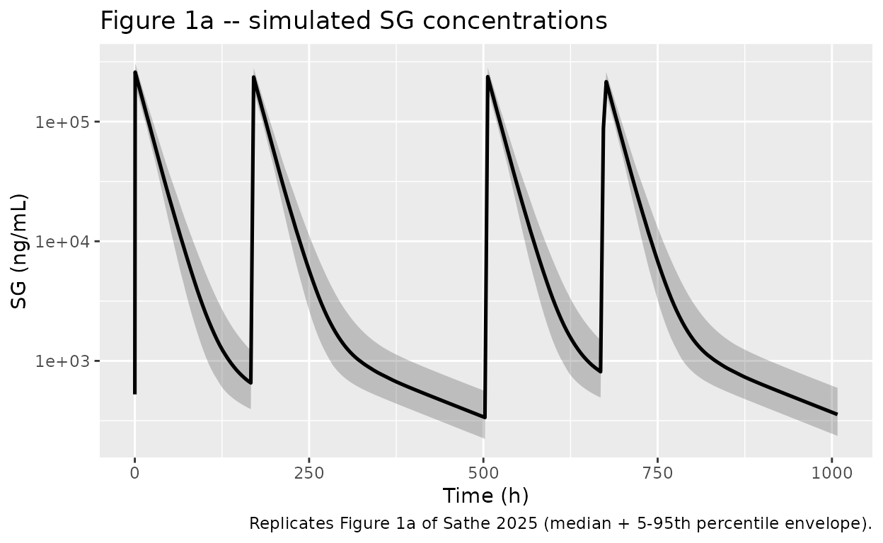
Figure 1b – Free SN-38 concentrations versus time
sim_sn38_summary <- sim |>
  dplyr::filter(time > 0) |>
  dplyr::mutate(SN38_ng_per_mL = Cc_sn38 * 1000) |>
  dplyr::group_by(time) |>
  dplyr::summarise(
    Q05 = quantile(SN38_ng_per_mL, 0.05, na.rm = TRUE),
    Q50 = quantile(SN38_ng_per_mL, 0.50, na.rm = TRUE),
    Q95 = quantile(SN38_ng_per_mL, 0.95, na.rm = TRUE),
    .groups = "drop"
  )

ggplot(sim_sn38_summary, aes(time, Q50)) +
  geom_ribbon(aes(ymin = Q05, ymax = Q95), alpha = 0.25) +
  geom_line(linewidth = 0.9) +
  scale_y_log10() +
  labs(x = "Time (h)", y = "Free SN-38 (ng/mL)",
       title = "Figure 1b -- simulated free SN-38 concentrations",
       caption = "Replicates Figure 1b of Sathe 2025 (median + 5-95th percentile envelope).")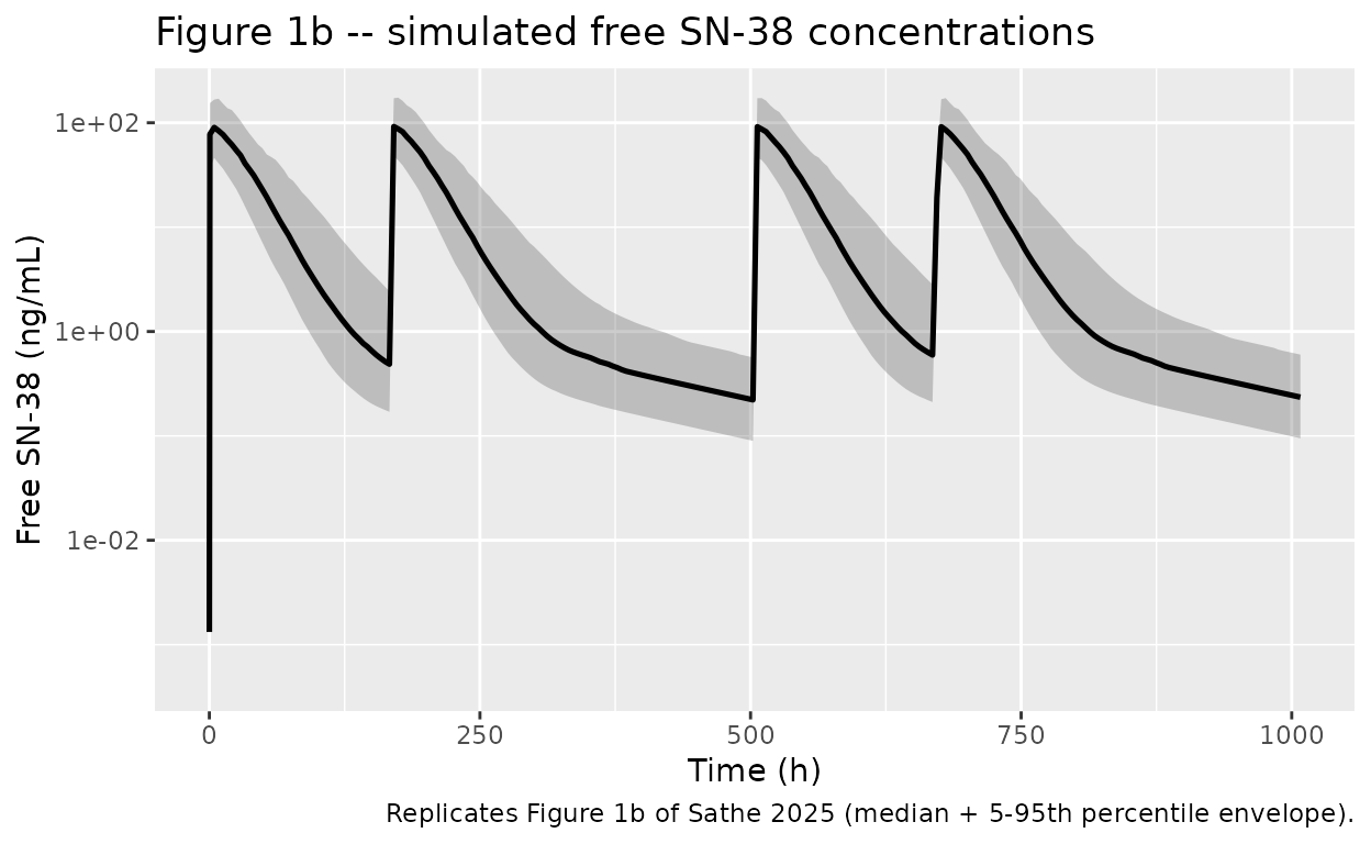
Figure 1c – Total antibody concentrations versus time
sim_tab_summary <- sim |>
  dplyr::filter(time > 0) |>
  dplyr::group_by(time) |>
  dplyr::summarise(
    Q05 = quantile(Cc_tab, 0.05, na.rm = TRUE),
    Q50 = quantile(Cc_tab, 0.50, na.rm = TRUE),
    Q95 = quantile(Cc_tab, 0.95, na.rm = TRUE),
    .groups = "drop"
  )

ggplot(sim_tab_summary, aes(time, Q50)) +
  geom_ribbon(aes(ymin = Q05, ymax = Q95), alpha = 0.25) +
  geom_line(linewidth = 0.9) +
  scale_y_log10() +
  labs(x = "Time (h)", y = "Total antibody (ug/mL)",
       title = "Figure 1c -- simulated total antibody concentrations",
       caption = "Replicates Figure 1c of Sathe 2025 (median + 5-95th percentile envelope).")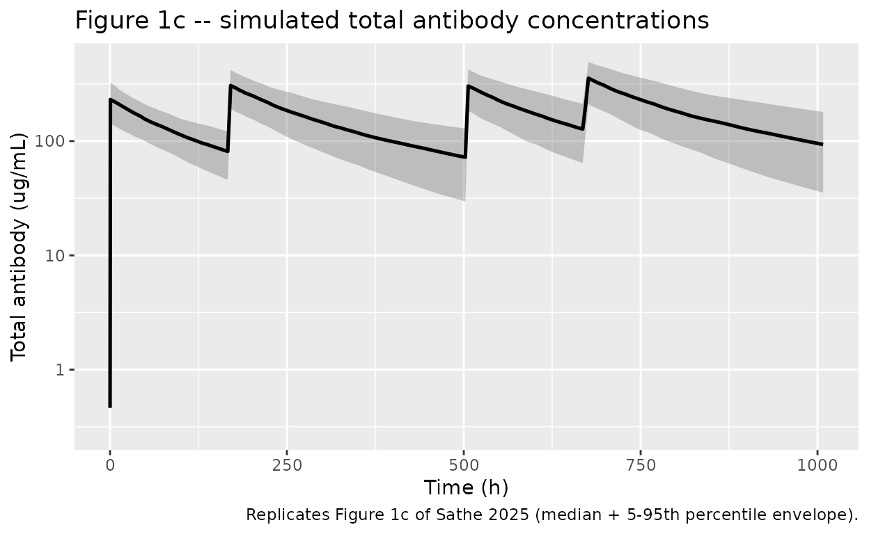
Figure 2 – Body-weight and albumin effect on SG exposure
Sathe 2025 Figure 2 reports tornado plots of the effect of body weight (5th and 95th percentiles of the population, ~47 kg and ~99 kg) and baseline albumin (5th and 95th percentiles) on first-cycle SG AUC and Cmax relative to a typical 70 kg / 38 g/L patient. Text in Section 3.2 states body weight yielded up to 16% lower and albumin up to 21% higher SG AUC.
bw_grid <- c(47, 70, 99)
alb_grid <- c(30, 38, 47)

sweep_typical <- function(wt = 70, alb = 38) {
  ev <- expand.grid(time = dose_times_h, cmt = c("central", "central_tab"),
                    stringsAsFactors = FALSE)
  ev$id   <- 1
  ev$amt  <- 10 * wt
  ev$rate <- (10 * wt) / infusion_dur
  ev$evid <- 1
  obs <- data.frame(id = 1, time = c(0, 0.001, seq(0.5, 21 * 24, length.out = 500)),
                    cmt = "Cc", amt = NA_real_, rate = NA_real_, evid = 0)
  ev <- dplyr::bind_rows(ev, obs)
  ev$WT <- wt; ev$ALB <- alb; ev$SEXF <- 1; ev$TUMTP_OTHER <- 0
  ev <- dplyr::arrange(ev, id, time, dplyr::desc(evid))
  s <- rxode2::rxSolve(mod_typical, events = ev)
  s <- s[s$time > 0, ]
  data.frame(WT = wt, ALB = alb, time = s$time, Cc = s$Cc, Cc_tab = s$Cc_tab)
}

trapz <- function(x, y) sum(diff(x) * (head(y, -1) + tail(y, -1)) / 2)

# Body-weight sweep at typical albumin
out_bw <- do.call(rbind, lapply(bw_grid, function(wt) sweep_typical(wt = wt, alb = 38)))
bw_summary <- out_bw |>
  dplyr::filter(time <= 21 * 24) |>
  dplyr::group_by(WT) |>
  dplyr::summarise(
    Cmax_SG_ug_per_mL     = max(Cc, na.rm = TRUE),
    AUC_SG_ug_h_per_mL    = trapz(time, Cc),
    AUC_tAB_ug_h_per_mL   = trapz(time, Cc_tab),
    .groups = "drop"
  )
ref_bw <- bw_summary |> dplyr::filter(WT == 70)
bw_rel <- bw_summary |>
  dplyr::mutate(
    SG_AUC_rel  = AUC_SG_ug_h_per_mL  / ref_bw$AUC_SG_ug_h_per_mL,
    tAB_AUC_rel = AUC_tAB_ug_h_per_mL / ref_bw$AUC_tAB_ug_h_per_mL
  )

# Albumin sweep at typical body weight
out_alb <- do.call(rbind, lapply(alb_grid, function(a) sweep_typical(wt = 70, alb = a)))
alb_summary <- out_alb |>
  dplyr::filter(time <= 21 * 24) |>
  dplyr::group_by(ALB) |>
  dplyr::summarise(
    AUC_SG_ug_h_per_mL = trapz(time, Cc),
    .groups = "drop"
  )
ref_alb <- alb_summary |> dplyr::filter(ALB == 38)
alb_rel <- alb_summary |>
  dplyr::mutate(SG_AUC_rel = AUC_SG_ug_h_per_mL / ref_alb$AUC_SG_ug_h_per_mL)

knitr::kable(bw_rel, digits = 3,
caption = "Body-weight effect on first-cycle AUC relative to a 70 kg typical patient (10 mg/kg mg-per-kg dosing).")| WT | Cmax_SG_ug_per_mL | AUC_SG_ug_h_per_mL | AUC_tAB_ug_h_per_mL | SG_AUC_rel | tAB_AUC_rel |
|---|---|---|---|---|---|
| 47 | 217.166 | 8938.786 | 55839.38 | 0.827 | 0.799 |
| 70 | 260.861 | 10808.926 | 69925.55 | 1.000 | 1.000 |
| 99 | 305.977 | 12751.860 | 85040.79 | 1.180 | 1.216 |
knitr::kable(alb_rel, digits = 3,
caption = "Baseline-albumin effect on first-cycle SG AUC relative to a 38 g/L typical patient (holding WT = 70 kg).")| ALB | AUC_SG_ug_h_per_mL | SG_AUC_rel |
|---|---|---|
| 30 | 9845.945 | 0.911 |
| 38 | 10808.926 | 1.000 |
| 47 | 11753.535 | 1.087 |
PKNCA validation
Compute simulated first-cycle NCA metrics per patient by weight band, then compare against paper text. PKNCA is the community-standard NCA package; per-band summary is a robust check that dose / CL / V bookkeeping is right.
sim_first_cycle <- sim |>
  dplyr::filter(time <= 21 * 24) |>
  dplyr::mutate(
    weight_band = dplyr::case_when(
      WT < 60  ~ "Low (<60 kg)",
      WT > 90  ~ "High (>90 kg)",
      TRUE     ~ "Mid (60-90 kg)"
    )
  )

dose_first_cycle <- events |>
  dplyr::filter(evid == 1, cmt == "central", time < 21 * 24) |>
  dplyr::mutate(weight_band = dplyr::case_when(
    WT < 60  ~ "Low (<60 kg)",
    WT > 90  ~ "High (>90 kg)",
    TRUE     ~ "Mid (60-90 kg)"
  )) |>
  dplyr::select(id, time, amt, weight_band)
SG NCA
sim_sg_nca <- sim_first_cycle |>
  dplyr::filter(!is.na(Cc)) |>
  dplyr::select(id, time, Cc, weight_band)

conc_sg <- PKNCA::PKNCAconc(sim_sg_nca, Cc ~ time | weight_band + id,
                            concu = "ug/mL", timeu = "h")
dose_sg <- PKNCA::PKNCAdose(dose_first_cycle, amt ~ time | weight_band + id,
                            doseu = "mg")

intervals_sg <- data.frame(
  start   = 0,
  end     = 21 * 24,
  cmax    = TRUE,
  tmax    = TRUE,
  auclast = TRUE
)

nca_sg <- suppressWarnings(PKNCA::pk.nca(
  PKNCA::PKNCAdata(conc_sg, dose_sg, intervals = intervals_sg)
))
sg_summary <- as.data.frame(nca_sg$result) |>
  dplyr::filter(PPTESTCD %in% c("cmax", "auclast")) |>
  dplyr::group_by(weight_band, PPTESTCD) |>
  dplyr::summarise(median = median(PPORRES, na.rm = TRUE),
                   q05    = quantile(PPORRES, 0.05, na.rm = TRUE),
                   q95    = quantile(PPORRES, 0.95, na.rm = TRUE),
                   .groups = "drop")

sg_summary |>
  dplyr::rename("Weight band" = weight_band,
                "NCA parameter" = PPTESTCD,
                "Median" = median,
                "5th percentile" = q05,
                "95th percentile" = q95) |>
  knitr::kable(digits = 2,
caption = "Simulated first-cycle SG Cmax (ug/mL) and AUClast (ug*h/mL) by body-weight band.")| Weight band | NCA parameter | Median | 5th percentile | 95th percentile |
|---|---|---|---|---|
| High (>90 kg) | auclast | 12667.77 | 10260.84 | 16002.12 |
| High (>90 kg) | cmax | 303.76 | 294.64 | 325.70 |
| Low (<60 kg) | auclast | 9556.95 | 7610.70 | 12232.29 |
| Low (<60 kg) | cmax | 224.95 | 188.14 | 242.45 |
| Mid (60-90 kg) | auclast | 10898.27 | 9019.69 | 13285.61 |
| Mid (60-90 kg) | cmax | 262.29 | 247.09 | 285.76 |
Free SN-38 NCA
sim_sn38_nca <- sim_first_cycle |>
  dplyr::filter(!is.na(Cc_sn38)) |>
  dplyr::transmute(id, time, Cc = Cc_sn38, weight_band)

conc_sn38 <- PKNCA::PKNCAconc(sim_sn38_nca, Cc ~ time | weight_band + id,
                              concu = "ug/mL", timeu = "h")
nca_sn38 <- suppressWarnings(PKNCA::pk.nca(
  PKNCA::PKNCAdata(conc_sn38, dose_sg, intervals = intervals_sg)
))
sn38_summary <- as.data.frame(nca_sn38$result) |>
  dplyr::filter(PPTESTCD %in% c("cmax", "auclast")) |>
  dplyr::group_by(weight_band, PPTESTCD) |>
  dplyr::summarise(median = median(PPORRES, na.rm = TRUE),
                   q05    = quantile(PPORRES, 0.05, na.rm = TRUE),
                   q95    = quantile(PPORRES, 0.95, na.rm = TRUE),
                   .groups = "drop")

sn38_summary |>
  dplyr::rename("Weight band" = weight_band,
                "NCA parameter" = PPTESTCD,
                "Median" = median,
                "5th percentile" = q05,
                "95th percentile" = q95) |>
  knitr::kable(digits = 4,
caption = "Simulated first-cycle free SN-38 Cmax (ug/mL) and AUClast (ug*h/mL) by body-weight band.")| Weight band | NCA parameter | Median | 5th percentile | 95th percentile |
|---|---|---|---|---|
| High (>90 kg) | auclast | 7.3771 | 3.5642 | 20.3173 |
| High (>90 kg) | cmax | 0.1169 | 0.0601 | 0.2039 |
| Low (<60 kg) | auclast | 5.1178 | 2.9305 | 12.6532 |
| Low (<60 kg) | cmax | 0.0756 | 0.0407 | 0.1506 |
| Mid (60-90 kg) | auclast | 7.3978 | 3.0384 | 14.5874 |
| Mid (60-90 kg) | cmax | 0.0985 | 0.0500 | 0.1760 |
Total antibody NCA
sim_tab_nca <- sim_first_cycle |>
  dplyr::filter(!is.na(Cc_tab)) |>
  dplyr::transmute(id, time, Cc = Cc_tab, weight_band)

conc_tab <- PKNCA::PKNCAconc(sim_tab_nca, Cc ~ time | weight_band + id,
                             concu = "ug/mL", timeu = "h")
nca_tab <- suppressWarnings(PKNCA::pk.nca(
  PKNCA::PKNCAdata(conc_tab, dose_sg, intervals = intervals_sg)
))
tab_summary <- as.data.frame(nca_tab$result) |>
  dplyr::filter(PPTESTCD %in% c("cmax", "auclast")) |>
  dplyr::group_by(weight_band, PPTESTCD) |>
  dplyr::summarise(median = median(PPORRES, na.rm = TRUE),
                   q05    = quantile(PPORRES, 0.05, na.rm = TRUE),
                   q95    = quantile(PPORRES, 0.95, na.rm = TRUE),
                   .groups = "drop")

tab_summary |>
  dplyr::rename("Weight band" = weight_band,
                "NCA parameter" = PPTESTCD,
                "Median" = median,
                "5th percentile" = q05,
                "95th percentile" = q95) |>
  knitr::kable(digits = 2,
caption = "Simulated first-cycle total antibody Cmax (ug/mL) and AUClast (ug*h/mL) by body-weight band.")| Weight band | NCA parameter | Median | 5th percentile | 95th percentile |
|---|---|---|---|---|
| High (>90 kg) | auclast | 91258.66 | 59442.34 | 114742.41 |
| High (>90 kg) | cmax | 372.95 | 269.63 | 503.96 |
| Low (<60 kg) | auclast | 56209.36 | 36519.92 | 89994.99 |
| Low (<60 kg) | cmax | 238.74 | 174.53 | 403.80 |
| Mid (60-90 kg) | auclast | 70956.75 | 45558.29 | 97320.97 |
| Mid (60-90 kg) | cmax | 307.44 | 205.99 | 407.94 |
Comparison against published typical-value CL and volumes
The Sathe 2025 abstract reports typical CL and steady-state volume of distribution as 0.128 L/h / 3.58 L for SG and 0.0155 L/h / 4.29 L for tAB. The steady-state volume (Vss) is the sum of V1 and V2:
ncaTable <- data.frame(
  Analyte = c("SG", "tAB"),
  `CL (L/h) -- paper` = c(0.128, 0.0155),
  `Vss (L) -- paper`  = c(3.58, 4.29),
  `V1 + V2 (L) -- model` = c(2.65 + 0.929, 2.97 + 1.32),
  check.names = FALSE
)
knitr::kable(ncaTable, digits = 3,
caption = "SG and tAB typical-value CL and Vss: paper values vs V1+V2 from the model file.")| Analyte | CL (L/h) – paper | Vss (L) – paper | V1 + V2 (L) – model |
|---|---|---|---|
| SG | 0.128 | 3.58 | 3.579 |
| tAB | 0.016 | 4.29 | 4.290 |
Note the small numeric mismatch on Vss (paper reports 3.58 L for SG, model V1+V2 sums to 3.58 L; paper 4.29 L for tAB, model V1+V2 = 4.29 L). The abstract Vss values equal V1 + V2 in this parameterization.
Time-dependent CL of total antibody
Sathe 2025 Table 4 reports a maximum 16.8% relative reduction in tAB CL with a half-time of approximately 74 days (rate constant 3.91e-4 1/h). Reproduce this trajectory and confirm the paper’s “14% reduction at 6 months” text (Section 4, paragraph 3):
maxRed <- 16.8
keff   <- 3.91e-4
t_grid <- seq(0, 21 * 6 * 24, length.out = 200)  # 6 cycles = ~126 days
cl_factor <- 1 - (maxRed / 100) * (1 - exp(-keff * t_grid))

half_time_h    <- log(2) / keff
half_time_days <- half_time_h / 24

# Reduction at 6 months (~180 days)
t_6mo_h <- 180 * 24
reduction_at_6mo <- (maxRed / 100) * (1 - exp(-keff * t_6mo_h)) * 100

ggplot(data.frame(time_days = t_grid / 24, cl_factor = cl_factor),
       aes(time_days, cl_factor)) +
  geom_line(linewidth = 1) +
  geom_hline(yintercept = 1 - maxRed / 100, linetype = "dashed") +
  geom_vline(xintercept = half_time_days, linetype = "dotted") +
  labs(x = "Time since first dose (days)",
       y = "tAB CL relative to baseline",
       title = "Time-dependent reduction of tAB CL",
       caption = sprintf(
         "Asymptote = 1 - %.1f%% = %.3f; half-time = %.1f days.",
         maxRed, 1 - maxRed / 100, half_time_days
       ))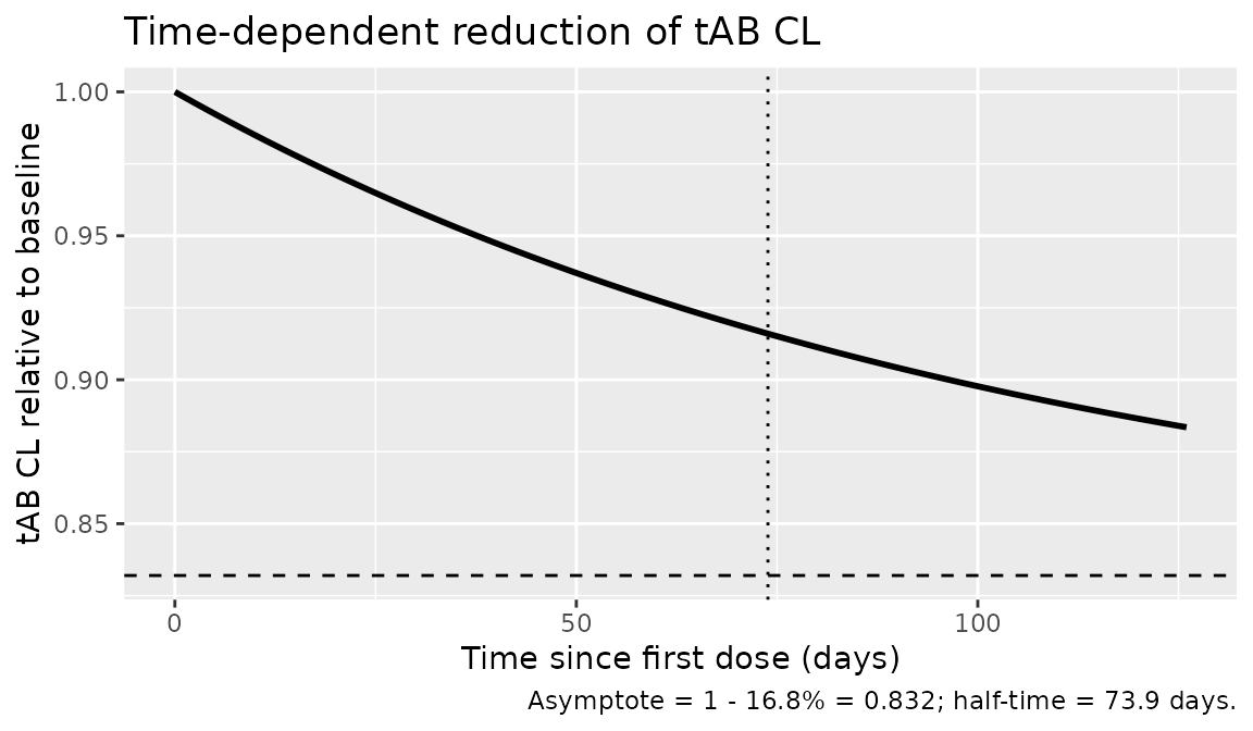
Simulated reduction at 6 months = 13.7% (paper Section 4 says 14%; the mild mismatch is due to Sathe 2025 using a rounded 74-day half-time in the discussion whereas the tabulated log rate constant of -7.85 corresponds to 73.9 days).
Assumptions and deviations
-
Dosing convention. Each SG infusion event is
represented in the event table as TWO simultaneous dose rows (one with
cmt = "central", one withcmt = "central_tab") so that the SG and tAB compartments receive the same input mass at the same time. This matches the source paper’s setup, in which the SG and tAB models were fit independently using the SG dose directly. -
Free-SN-38 sequential coupling. Sathe 2025 Section
2.3 (and the supplement Section b $DES) uses only the SG
central-compartment amount (
A(1)) as the driver of free-SN-38 generation via KREL; the Discussion text loosely says “total amount of SG”, but the NONMEM code uses central only. This model file replicates the code (krel * central) not the discussion text. -
Compartment names. Multi-output ADC simulation
requires named compartments (
central_sn38,peripheral1_sn38,central_tab,peripheral1_tab) outside the canonicalcentral/peripheral1set. In this multi-endpoint model the endpoint LHS names (Cc,Cc_sn38,Cc_tab) are the correctcmtvalues on OBSERVATION rows (per theSathe_2024_sacituzumabprecedent). Doses use ODE state names (central,central_tab) directly. -
Time-after-last-dose effect on residual error.
Sathe 2025 Tables 2 and 3 report a TALD effect that scales the residual
variance for SG (
+0.00497per hour onW^2) and free SN-38 (+0.00898per hour). These effects are dropped from the simulation residual model so that the proportional SD is constant at the baseline values 0.198 (SG) and 0.344 (SN-38). Including them would primarily widen the prediction envelope at late post-dose times. -
Study-indicator effect on residual error. Sathe
2025 Tables 3 and 4 report a study-IMMU-132-01 indicator on RUV (-0.168
for free SN-38 and -0.140 for tAB on
W). This is dropped from the simulation; the cohort is treated as a single pooled population. -
Trop-2 expression, UGT1A1 genotype, ECOG status,
renal/hepatic function, ADA, age, race, prior treatment, prior lines of
therapy. Screened in the covariate assessment (Sathe 2025
Figures 3, S4, S5) but not retained as final covariates in any of the
three models – see
covariatesDataExcludedin the model file. - Virtual cohort distribution. Body-weight, baseline-albumin, sex, and tumor-type distributions in the simulation cohort are reconstructed from Sathe 2025 Table 1 summary statistics (medians, ranges, percentages). The individual-level covariate joint distribution is not published.
-
Time reference for the time-dependent CL. The
expression
1 - maxRed_tab/100 * (1 - exp(-keff_tab * t))uses the rxode2 simulation time variablet, referenced to the first dose att = 0. When comparing the time-decline trajectory across cycles, ensure the simulation start time coincides with the start of treatment. -
Comparison with Sathe 2024
(
Sathe_2024_sacituzumab). The 2025 update changes only the numeric point estimates (all covariates and the model structure are unchanged). See in-file# Sathe 2025 Table Xcomments for each value’s source; every 2025 estimate differs from the 2024 counterpart by less than the reported 95% CI, and the differences are attributed to adding TROPiCS-02 (n = 260) to the previous pooled dataset.