Dexamethasone contact-lens ocular PK in the rabbit (Toffoletto 2023)
Source:vignettes/articles/Toffoletto_2023_dexamethasone_rabbit.Rmd
Toffoletto_2023_dexamethasone_rabbit.RmdModel and source
ui <- rxode2::rxode(readModelDb("Toffoletto_2023_dexamethasone_rabbit"))- Citation: Toffoletto N, Saramago B, Serro AP, Chauhan A. A Physiology-Based Mathematical Model to Understand Drug Delivery from Contact Lenses to the Back of the Eye. Pharm Res. 2023;40(8):1939-1951. doi:10.1007/s11095-023-03560-7. Validation data: Ross AE et al. Topical sustained drug delivery to the retina with a drug-eluting contact lens. Biomaterials. 2019;217:119285. doi:10.1016/j.biomaterials.2019.119285.
- Description: Preclinical (rabbit). Physiology-based ocular PK model of dexamethasone released from a drug-eluting soft contact lens (Ross 2019 sandwich lens), with well-mixed tear film, lumped sclera-choroid, retina, vitreous humour and aqueous humour (plus stroma) compartments. Transport across each barrier is area x permeability x the difference of the partition-corrected concentrations; drug leaves by tear drainage, palpebral-conjunctival uptake, choroidal blood-flow clearance, uveoscleral outflow and aqueous-humour turnover. The lens is a first-order depot (Eqs. 12-13): a fraction F of the released drug crosses the cornea directly into the aqueous humour and the rest enters the tears (Eqs. 10-11). Deterministic (no IIV or residual error); every value is a literature or hand-tuned input, not a statistical estimate.
- Article: https://doi.org/10.1007/s11095-023-03560-7 (open access; PMC10447275)
- Supplement: Electronic Supplementary Material 1 (Supplementary Figs. S1-S2, Supplementary Table S1), available from the article page.
Toffoletto et al. built a physiology-based ocular model to follow a
drug from a therapeutic soft contact lens into the tear film, the sclera
and choroid, the retina, the vitreous humour and the aqueous humour.
Transport across each barrier is the exposed area times the barrier
permeability times the difference of the partition-corrected
concentrations (Eqs. 2-6). The general form treats the lens as a
diffusion slab (Eq. 1, a partial differential equation in the lens
thickness). For the only time-course data available, the dexamethasone
sandwich lens of Ross et al. (2019), release is governed by polymer
degradation rather than diffusion, so the authors replaced the lens
equation by the measured in-vitro release,
R = M_Released / T * exp(-t/T) (Eqs. 12-13), of which a
fraction F crosses the cornea into the aqueous humour and
the rest enters the tears (Eqs. 10-11). That validated form is the one
packaged here. The lens is a depot dosed with the released
amount M_Released; first-order release from it with rate
constant ka = 1/T reproduces Eq. 13 exactly.
Population
The model was not fitted to animals. Its anatomy (Table II) and
physiology (Table IV) are literature values for the rabbit eye, and its
drug-specific inputs (Table III) are literature permeabilities and
partition coefficients for dexamethasone, two of them
(K_ScCh, K_Ret) adjusted by hand during the
validation. It was compared against the rabbit data of Ross et
al. (2019), who measured dexamethasone in the aqueous humour, choroid,
sclera, retina and vitreous humour at 0.25, 1, 2, 5 and 7 days of
wearing the lens (3-5 eyes per time point in Fig. 3 of Toffoletto 2023).
The model describes one eye.
str(ui$population)
#> List of 6
#>  $ species      : chr "rabbit"
#>  $ n_subjects   : int NA
#>  $ n_studies    : int 1
#>  $ disease_state: chr "healthy"
#>  $ dose_range   : chr "One dexamethasone-eluting sandwich contact lens per eye, worn for 7 days; about 1.05 mg released in vitro over "| __truncated__
#>  $ notes        : chr "No animals were studied in Toffoletto 2023: the model is parameterised from rabbit physiology (Tables II and IV"| __truncated__
Source trace
| Equation / parameter | Value | Source location |
|---|---|---|
d/dt(depot), release ka * depot
|
n/a | Eqs. 12-13 |
d/dt(tear) |
n/a | Eq. 10 |
d/dt(sclera_choroid) |
n/a | Eq. 3 |
d/dt(retina) |
n/a | Eq. 4 |
d/dt(vitreous) |
n/a | Eq. 5 |
d/dt(aqueous_humour) |
n/a | Eq. 11 |
lka (1/T) |
log(1/2.55 day) | Supplementary Fig. S1, right panel, exponential fit (digitised) |
dose M_Released
|
1047 ug | Supplementary Fig. S1, right panel, exponential fit (digitised) |
f_aqueous_humour (F) |
0.0208 | Table III, 2.08 percent (Eq. 14) |
p_conj |
2.5e-6 cm/s | Table III |
p_rpe (P_ScCh-Ret) |
10e-6 cm/s | Table III |
p_ilm (P_Ret-Vit) |
13e-6 cm/s | Table III |
kp_sclera_choroid |
15 | Table III |
kp_retina |
10 | Table III |
kp_vitreous, kp_tear
|
1 | Table IV |
q_uveoscleral |
0.176 uL/min | Table IV |
q_vitreous_aqueous_humour |
0.19 uL/min | Table IV |
q_aqueous_humour |
4.2 uL/min | Table IV |
q_tear_drainage |
0.5 uL/min | Table IV |
cl_sclera_choroid |
1 mL/min | Table IV |
v_tear, v_vitreous,
v_sclera_choroid, v_retina,
v_aqueous_humour
|
0.007, 1.7, 0.361, 0.086, 0.325 mL | Table II |
a_globe, a_palpebral,
a_bulbar
|
8.6, 14, 3 cm^2 | Table II |
Digitised reference values
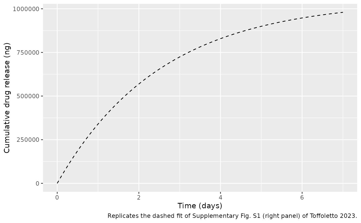
The paper prints neither the lens release constants nor any numerical
concentrations, so the maintainers digitised the figures. The release
curve of Supplementary Fig. S1 (the exponential fit of Eq. 12, drawn
dashed over the in-vitro data) gives
M_Released = 1.047e6 ng and T = 2.55 days. The
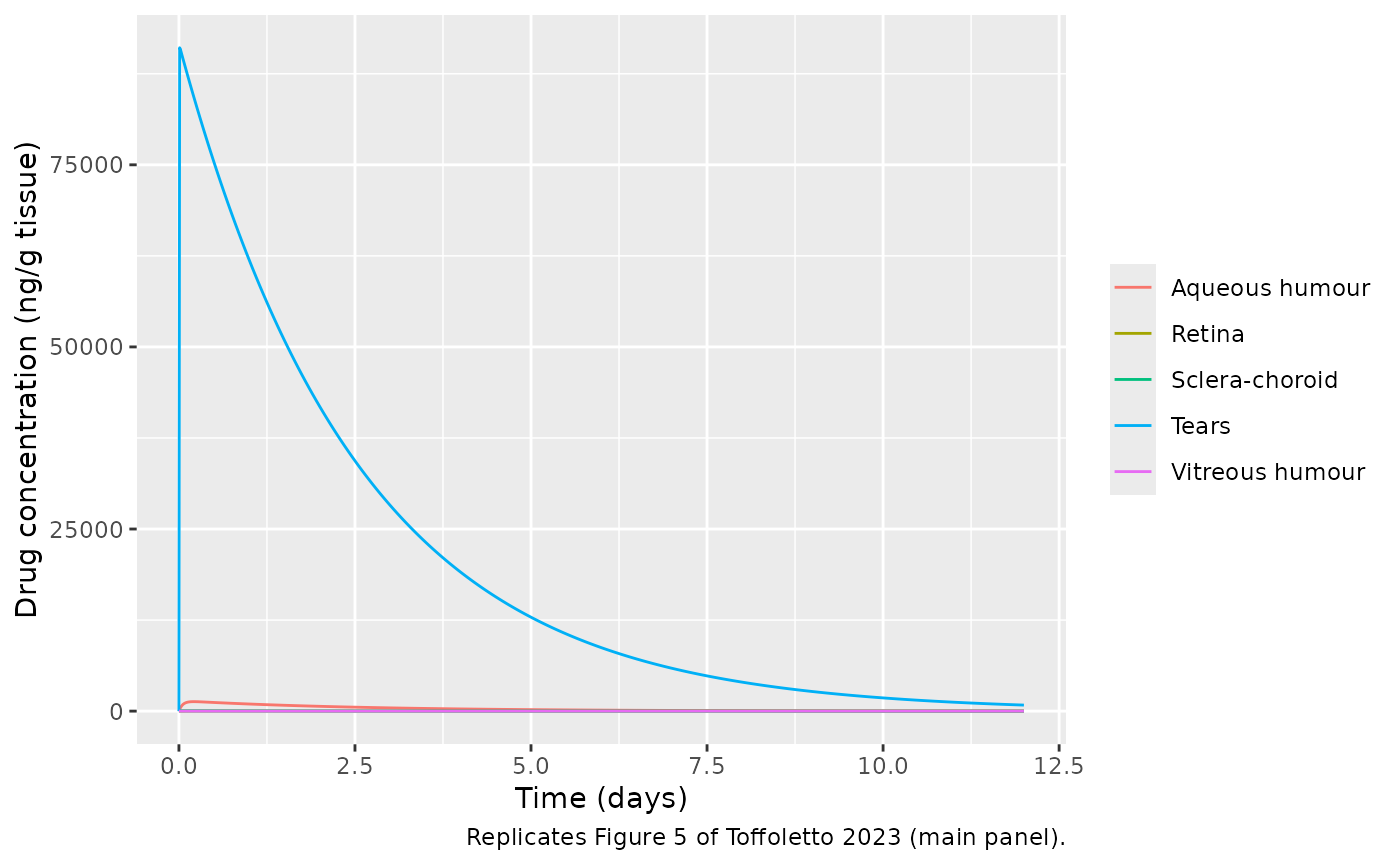
model curves of Fig. 3 (log scale) and Fig. 5 (linear scale, the same
simulation) give the values below; the tear curve of Fig. 5 is a single
exponential, 89,200 * exp(-t / 2.513 days) ng/mL.
fig3 <- tibble::tribble(
  ~tissue,            ~time, ~conc,
  "Aqueous humour",     0.5, 1140,
  "Aqueous humour",     1.5,  771,
  "Aqueous humour",     3.0,  419,
  "Aqueous humour",     4.0,  284,
  "Aqueous humour",     6.0,  130,
  "Aqueous humour",     8.0,   59.4,
  "Sclera-choroid",     0.15, 620,
  "Sclera-choroid",     4.0,  136,
  "Sclera-choroid",     6.0,   62.0,
  "Sclera-choroid",     8.0,   28.4,
  "Retina",             0.5,  376,
  "Retina",             1.5,  419,
  "Retina",             3.0,  272,
  "Retina",             4.0,  192,
  "Retina",             6.0,   87.8,
  "Retina",             8.0,   40.2,
  "Vitreous humour",    0.5,   30.3,
  "Vitreous humour",    1.5,   41.9,
  "Vitreous humour",    3.0,   28.4,
  "Vitreous humour",    4.0,   20.0,
  "Vitreous humour",    6.0,    9.17,
  "Vitreous humour",    8.0,    4.19
)
tear_fig5 <- function(t) 89200 * exp(-t / 2.513)
Simulation
One eye wearing the lens; the dose is the total amount released in
vitro. Observation rows sit on the tear state; rxode2
returns every concentration output on each row.
mod <- readModelDb("Toffoletto_2023_dexamethasone_rabbit")
m_released_ug <- 1047

times <- sort(unique(c(seq(0, 0.5, by = 0.01), seq(0.5, 12, by = 0.05), fig3$time)))
events <- rxode2::et(amt = m_released_ug, cmt = "depot") |>
  rxode2::et(time = times, cmt = "tear")

sim <- as.data.frame(rxode2::rxSolve(mod, events, rtol = 1e-10, atol = 1e-12))
if (is.null(sim$id)) sim$id <- 1L

tissue_cols <- c(
  Tears = "Ctear",
  "Aqueous humour" = "Caqueous_humour",
  "Sclera-choroid" = "Csclera_choroid",
  Retina = "Cretina",
  "Vitreous humour" = "Cvitreous"
)
sim_long <- sim |>
  dplyr::select(id, time, dplyr::all_of(unname(tissue_cols))) |>
  tidyr::pivot_longer(-c(id, time), names_to = "output", values_to = "Cc") |>
  dplyr::mutate(tissue = names(tissue_cols)[match(output, tissue_cols)])
Lens release
The depot reproduces the release fit of Supplementary Fig. S1 by
construction: the cumulative amount released is
M_Released * (1 - exp(-t/T)).
rel <- sim |> dplyr::mutate(released_ng = 1000 * (m_released_ug - depot))
stopifnot(
  max(abs(rel$released_ng - 1.047e6 * (1 - exp(-rel$time / 2.55)))) < 1
)
ggplot(rel |> dplyr::filter(time <= 7), aes(time, released_ng)) +
  geom_line(linetype = "dashed") +
  labs(
    x = "Time (days)", y = "Cumulative drug release (ng)",
    caption = "Replicates the dashed fit of Supplementary Fig. S1 (right panel) of Toffoletto 2023."
  )
Replicate published figures
Figure 5: all tissues, linear scale
ggplot(sim_long, aes(time, Cc, colour = tissue)) +
  geom_line() +
  labs(
    x = "Time (days)", y = "Drug concentration (ng/g tissue)", colour = NULL,
    caption = "Replicates Figure 5 of Toffoletto 2023 (main panel)."
  )
ggplot(sim_long |> dplyr::filter(tissue != "Tears"), aes(time, Cc, colour = tissue)) +
  geom_line() +
  labs(
    x = "Time (days)", y = "Drug concentration (ng/g tissue)", colour = NULL,
    caption = "Replicates the inset of Figure 5 of Toffoletto 2023."
  )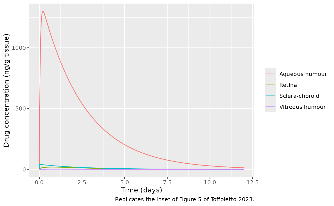
Figure 3: comparison with the published model curves
The packaged model (solid) against the model curves digitised from Fig. 3 (points). The tear film and the aqueous humour agree; the sclera-choroid, retina and vitreous do not (see Known discrepancy below). The dashed curves show the alternative reading of Eq. 3 described there.
# Alternative reading of Eq. 3: choroidal clearance acting on the
# partition-corrected concentration C_ScCh / K_ScCh, like every other
# outflow term of the sclera-choroid balance.
mod_alt <- rxode2::rxode(mod) |>
  rxode2::model(
    d/dt(sclera_choroid) <- q_uv * c_aq - q_uv * c_sc / kp_sclera_choroid +
      flux_bulbar - cl_sc * c_sc / kp_sclera_choroid - flux_rpe
  )
sim_alt <- as.data.frame(rxode2::rxSolve(mod_alt, events, rtol = 1e-10, atol = 1e-12))
if (is.null(sim_alt$id)) sim_alt$id <- 1L
sim_alt_long <- sim_alt |>
  dplyr::select(id, time, dplyr::all_of(unname(tissue_cols))) |>
  tidyr::pivot_longer(-c(id, time), names_to = "output", values_to = "Cc") |>
  dplyr::mutate(tissue = names(tissue_cols)[match(output, tissue_cols)])

fig3_tissues <- c("Aqueous humour", "Sclera-choroid", "Retina", "Vitreous humour")
ggplot(
  sim_long |> dplyr::filter(tissue %in% fig3_tissues, time >= 0.01, time <= 8),
  aes(time, Cc)
) +
  geom_line(aes(linetype = "Eq. 3 as printed (packaged)")) +
  geom_line(
    data = sim_alt_long |> dplyr::filter(tissue %in% fig3_tissues, time >= 0.01, time <= 8),
    aes(linetype = "Clearance on C_ScCh / K_ScCh")
  ) +
  geom_point(data = fig3, aes(time, conc), colour = "red") +
  facet_wrap(~tissue) +
  scale_y_log10(limits = c(1, 1e4)) +
  labs(
    x = "Time (days)", y = "Drug concentration (ng/g tissue)", linetype = NULL,
    caption = "Replicates Figure 3 of Toffoletto 2023; red points are its model curves, digitised."
  ) +
  theme(legend.position = "bottom")
#> Warning: Removed 129 rows containing missing values or values outside the scale range
#> (`geom_line()`).
#> Warning: Removed 4 rows containing missing values or values outside the scale range
#> (`geom_line()`).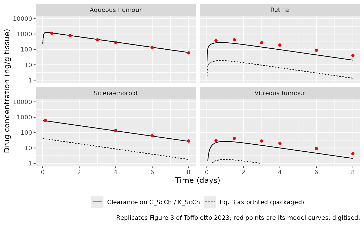
Quantitative checks
All checks below are deterministic (the model has no random effects), so their bounds only need to cover the digitisation error of the figures (a few percent).
at <- function(d, tis, t) {
  v <- d$Cc[d$tissue == tis & abs(d$time - t) < 1e-9]
  if (length(v) != 1L) stop("no unique simulated row for ", tis, " at ", t)
  v
}
cmp <- fig3 |>
  dplyr::rowwise() |>
  dplyr::mutate(
    printed = at(sim_long, tissue, time),
    alternative = at(sim_alt_long, tissue, time)
  ) |>
  dplyr::ungroup() |>
  dplyr::mutate(
    ratio_printed = printed / conc,
    ratio_alternative = alternative / conc
  )
cmp |>
  dplyr::rename(
    Tissue = tissue, "Time (day)" = time, "Fig. 3 (ng/g)" = conc,
    "Packaged model" = printed, "Alternative Eq. 3" = alternative,
    "Packaged / Fig. 3" = ratio_printed, "Alternative / Fig. 3" = ratio_alternative
  ) |>
knitr::kable(digits = 2, caption = "Simulated concentrations against the digitised Fig. 3 model curves.")| Tissue | Time (day) | Fig. 3 (ng/g) | Packaged model | Alternative Eq. 3 | Packaged / Fig. 3 | Alternative / Fig. 3 |
|---|---|---|---|---|---|---|
| Aqueous humour | 0.50 | 1140.00 | 1185.57 | 1186.44 | 1.04 | 1.04 |
| Aqueous humour | 1.50 | 771.00 | 801.09 | 802.15 | 1.04 | 1.04 |
| Aqueous humour | 3.00 | 419.00 | 444.85 | 445.49 | 1.06 | 1.06 |
| Aqueous humour | 4.00 | 284.00 | 300.54 | 300.97 | 1.06 | 1.06 |
| Aqueous humour | 6.00 | 130.00 | 137.18 | 137.37 | 1.06 | 1.06 |
| Aqueous humour | 8.00 | 59.40 | 62.61 | 62.70 | 1.05 | 1.06 |
| Sclera-choroid | 0.15 | 620.00 | 39.08 | 585.27 | 0.06 | 0.94 |
| Sclera-choroid | 4.00 | 136.00 | 8.64 | 129.80 | 0.06 | 0.95 |
| Sclera-choroid | 6.00 | 62.00 | 3.94 | 59.24 | 0.06 | 0.96 |
| Sclera-choroid | 8.00 | 28.40 | 1.80 | 27.04 | 0.06 | 0.95 |
| Retina | 0.50 | 376.00 | 17.96 | 268.43 | 0.05 | 0.71 |
| Retina | 1.50 | 419.00 | 16.28 | 244.34 | 0.04 | 0.58 |
| Retina | 3.00 | 272.00 | 9.45 | 141.96 | 0.03 | 0.52 |
| Retina | 4.00 | 192.00 | 6.40 | 96.16 | 0.03 | 0.50 |
| Retina | 6.00 | 87.80 | 2.92 | 43.91 | 0.03 | 0.50 |
| Retina | 8.00 | 40.20 | 1.33 | 20.04 | 0.03 | 0.50 |
| Vitreous humour | 0.50 | 30.30 | 1.49 | 22.14 | 0.05 | 0.73 |
| Vitreous humour | 1.50 | 41.90 | 1.66 | 24.84 | 0.04 | 0.59 |
| Vitreous humour | 3.00 | 28.40 | 0.98 | 14.78 | 0.03 | 0.52 |
| Vitreous humour | 4.00 | 20.00 | 0.67 | 10.02 | 0.03 | 0.50 |
| Vitreous humour | 6.00 | 9.17 | 0.30 | 4.58 | 0.03 | 0.50 |
| Vitreous humour | 8.00 | 4.19 | 0.14 | 2.09 | 0.03 | 0.50 |
tear_ratio <- sapply(c(1, 4, 8), function(t) at(sim_long, "Tears", t) / tear_fig5(t))
tear_ratio
#> [1] 1.032837 1.050883 1.075436

stopifnot(
  # Tears: the release constants and the tear outflows (Q_Drain, P_Conj x
  # A_Palp, P_Conj x A_Bulb) set this level. Measured 1.03, 1.05, 1.08 at
  # days 1, 4, 8: the Fig. 5 curve decays with T = 2.51 days against the
  # 2.55 days of Supplementary Fig. S1, so the ratio drifts up with time.
  all(abs(tear_ratio - 1) < 0.10),
  # Aqueous humour: F, Q_Aq and the release; measured 1.04-1.06.
  all(abs(cmp$ratio_printed[cmp$tissue == "Aqueous humour"] - 1) < 0.15)
)
PKNCA validation
PKNCA on each output, grouped by tissue. The paper reports no NCA
table; the reference values are the peaks digitised from Fig. 5 and, for
the aqueous humour, the area under the exponential fit of Supplementary
Fig. S1 (1636.7 * exp(-5e-6 t), t in seconds), which the
authors used in Eq. 14 to derive F: 1636.7 / 5e-6 ng s/mL =
3789 ng day/mL.
conc_nca <- sim_long |>
  dplyr::filter(!is.na(Cc)) |>
  dplyr::mutate(Cc = pmax(Cc, 0)) |>
  dplyr::select(id, time, Cc, tissue)
stopifnot(all(conc_nca$time[!duplicated(conc_nca[, c("id", "tissue")])] == 0))

dose_nca <- conc_nca |>
  dplyr::distinct(id, tissue) |>
  dplyr::mutate(time = 0, amt = m_released_ug)

conc_obj <- PKNCA::PKNCAconc(conc_nca, Cc ~ time | tissue + id)
dose_obj <- PKNCA::PKNCAdose(dose_nca, amt ~ time | tissue + id)
intervals <- data.frame(
  start = 0, end = Inf,
  cmax = TRUE, tmax = TRUE, aucinf.obs = TRUE, half.life = TRUE
)
nca_res <- PKNCA::pk.nca(PKNCA::PKNCAdata(conc_obj, dose_obj, intervals = intervals))

reference <- tibble::tribble(
  ~tissue,            ~PPTESTCD,    ~PPORRES,
  "Tears",            "cmax",       89200,
  "Tears",            "half.life",  2.513 * log(2),
  "Aqueous humour",   "cmax",       1234,
  "Aqueous humour",   "tmax",       0.22,
  "Aqueous humour",   "aucinf.obs", 1636.7 / 5e-6 / 86400,
  "Sclera-choroid",   "cmax",       611,
  "Retina",           "cmax",       447,
  "Retina",           "tmax",       1.02,
  "Vitreous humour",  "cmax",       42,
  "Vitreous humour",  "tmax",       1.18
)

nca_cmp <- nlmixr2lib::ncaComparisonTable(
  simulated = nca_res,
  reference = reference,
  by = "tissue",
  units = c(cmax = "ng/mL", tmax = "day", aucinf.obs = "ng*day/mL", half.life = "day"),
  tolerance_pct = 20
)
knitr::kable(
  nca_cmp,
  caption = paste(
    "Simulated vs. digitised published values (Fig. 5 peaks; Supplementary",
    "Fig. S1 aqueous AUC). * differs by more than 20 percent."
  )
)| NCA parameter | tissue | Reference | Simulated | % diff |
|---|---|---|---|---|
| Cmax (ng/mL) | Tears | 89200 | 91100 | +2.1% |
| Cmax (ng/mL) | Aqueous humour | 1230 | 1300 | +5.3% |
| Cmax (ng/mL) | Sclera-choroid | 611 | 41 | -93.3%* |
| Cmax (ng/mL) | Retina | 447 | 18.7 | -95.8%* |
| Cmax (ng/mL) | Vitreous humour | 42 | 1.79 | -95.7%* |
| Tmax (day) | Aqueous humour | 0.22 | 0.21 | -4.5% |
| Tmax (day) | Retina | 1.02 | 0.75 | -26.5%* |
| Tmax (day) | Vitreous humour | 1.18 | 1 | -15.3% |
| AUC0-∞ (obs) (ng*day/mL) | Aqueous humour | 3790 | 3600 | -5.0% |
| t½ (day) | Tears | 1.74 | 1.77 | +1.5% |
The tear film and aqueous humour agree within a few percent,
including the aqueous-humour AUC that the authors used to derive
F (F = Q_Aq x AUC / M_Released): the simulated
AUC is about 5 percent below the Supplementary Fig. S1 value, consistent
with the one-significant-figure rate constant (5E-06)
printed on that fit. The sclera-choroid, retina and vitreous peaks are
starred; see below.
Known discrepancy: sclera-choroid, retina and vitreous
Eq. 3 removes drug from the sclera-choroid by choroidal blood flow as
Clearance_ScCh x C_ScCh, with
Clearance_ScCh = 1 mL/min (Table IV). Solved as printed,
the sclera-choroid concentration is about 16 times below the paper’s own
Fig. 3 and Fig. 5 curves, and the retina and vitreous (fed from the
sclera-choroid) are 20-35 times below. Every other outflow of the
sclera-choroid balance acts on the partition-corrected concentration
C_ScCh / K_ScCh; applying the choroidal clearance to that
concentration as well (equivalently, a clearance of 1/15 mL/min on
C_ScCh) reproduces the published sclera-choroid curve
within about 6 percent, but still leaves the retina and vitreous at
0.5-0.7 times the published curves. No single reading of the printed
equations and tables reproduces all five published curves, so the
package keeps Eq. 3 and Table IV exactly as printed; the alternative
reading is shown above for comparison. The checks below pin both
behaviours so that any later change to the model has to revisit this
section.
r <- function(col, tis) cmp[[col]][cmp$tissue == tis]
stopifnot(
  # As printed: sclera-choroid ratios measured 0.06; retina 0.03-0.05;
  # vitreous 0.03-0.05.
  all(r("ratio_printed", "Sclera-choroid") < 0.2),
  all(r("ratio_printed", "Retina") < 0.2),
  all(r("ratio_printed", "Vitreous humour") < 0.2),
  # Alternative reading: sclera-choroid measured 0.94-0.96; retina and
  # vitreous measured 0.50-0.73.
  all(abs(r("ratio_alternative", "Sclera-choroid") - 1) < 0.2),
  all(r("ratio_alternative", "Retina") < 0.85),
  all(r("ratio_alternative", "Vitreous humour") < 0.85)
)
Other drugs (Supplementary Table S1)
The authors also compared the model with single-study data for
melatonin, dexamethasone (Bengani 2020 lens), latanoprost, ofloxacin and
pravastatin (Fig. 4), changing only the drug- and lens-specific inputs
of Supplementary Table S1. The release constants of those lenses
(M_Released, T, or the diffusion-lens inputs
D_SCL, H, K_SCL) are not
reported, so those scenarios cannot be reproduced here; the drug inputs
can be swapped into the packaged model with rxode2::ini()
once a release profile is available.
table_s1 <- tibble::tribble(
  ~drug,                          ~p_conj, ~p_rpe, ~p_ilm, ~kp_sclera_choroid, ~kp_retina, ~f_aqueous_humour,
  "Dexamethasone (Bengani 2020)", 2.5e-6,  10e-6,  13e-6,  15,                 10,         0.0349,
  "Melatonin",                    2.5e-6,  10e-6,  13e-6,  15,                 10,         0.0293,
  "Latanoprost",                  3.0e-6,  10e-6,  13e-6,  17,                 11,         0.0208,
  "Ofloxacin",                    2.5e-7,   5e-6,   7e-6,   7,                  5,         0.0707,
  "Pravastatin",                  2.5e-7,   3e-6,   4e-6,   3,                  3,         0.0787
)
table_s1 |>
  dplyr::mutate(dplyr::across(c(p_conj, p_rpe, p_ilm), function(x) formatC(x, format = "e", digits = 1))) |>
knitr::kable(caption = "Supplementary Table S1 drug-specific inputs (permeabilities in cm/s).")| drug | p_conj | p_rpe | p_ilm | kp_sclera_choroid | kp_retina | f_aqueous_humour |
|---|---|---|---|---|---|---|
| Dexamethasone (Bengani 2020) | 2.5e-06 | 1.0e-05 | 1.3e-05 | 15 | 10 | 0.0349 |
| Melatonin | 2.5e-06 | 1.0e-05 | 1.3e-05 | 15 | 10 | 0.0293 |
| Latanoprost | 3.0e-06 | 1.0e-05 | 1.3e-05 | 17 | 11 | 0.0208 |
| Ofloxacin | 2.5e-07 | 5.0e-06 | 7.0e-06 | 7 | 5 | 0.0707 |
| Pravastatin | 2.5e-07 | 3.0e-06 | 4.0e-06 | 3 | 3 | 0.0787 |
# Example: the ofloxacin inputs, ready for a user-supplied release profile.
mod_oflox <- rxode2::rxode(mod) |>
  rxode2::ini(
    p_conj = 2.5e-7, p_rpe = 5e-6, p_ilm = 7e-6,
    kp_sclera_choroid = 7, kp_retina = 5, f_aqueous_humour = 0.0707
  )
#> ℹ change initial estimate of `p_conj` to `2.5e-07`
#> ℹ change initial estimate of `p_rpe` to `5e-06`
#> ℹ change initial estimate of `p_ilm` to `7e-06`
#> ℹ change initial estimate of `kp_sclera_choroid` to `7`
#> ℹ change initial estimate of `kp_retina` to `5`
#> ℹ change initial estimate of `f_aqueous_humour` to `0.0707`
stopifnot(isTRUE(all.equal(unname(mod_oflox$theta["kp_retina"]), 5)))
Assumptions and deviations
-
Release constants digitised.
M_ReleasedandTare not printed. The maintainers digitised the dashed exponential fit of Supplementary Fig. S1 (right panel) and fitted Eq. 12 to the digitised curve:M_Released = 1.047e6 ng,T = 2.55 days. Two independent checks agree: the tear curve of Fig. 5 decays with a time constant of 2.51 days, and the tear and aqueous-humour levels it implies are within 2-8 percent of the simulation. Using the 7-day in-vitro total of about 1.1e6 ng instead reproduces the printedF = 2.08percent more closely through Eq. 14, so the released amount is uncertain by about 5 percent. -
Ffor the Ross 2019 lens. Table III givesF = 2.08percent for this data set, while Supplementary Table S1 gives 3.49 percent for the Bengani 2020 dexamethasone lens and 2.08 percent for latanoprost. The Table III value is used here; the Bengani value belongs to a different lens. - Sclera-choroid clearance kept as printed. See Known discrepancy. The printed Eq. 3 and Table IV value under-predict the published sclera-choroid, retina and vitreous curves; the alternative reading is shown but not packaged.
-
Corneal epithelium not included. Eq. 7 needs the
partition coefficients
K_Ep/AqandK_Ep/t, which the paper does not report; the corneal-epithelium concentration is therefore not an output. - Diffusion-lens form not included. Eqs. 1, 2, 6, 8 and 9 describe diffusion through the lens thickness (a partial differential equation). The paper gives no lens diffusivity, thickness or lens partition coefficient, and its validation uses the release-rate form instead.
-
K_Aqnot used. Table IV listsK_Aq = 1, but it appears in none of the validated equations (Eqs. 3-5, 10, 11), so the model does not carry it. - Concentration units. Outputs are ng/mL; the paper reports ng/g tissue, which is the same number at unit tissue density.
- No variability. The model is deterministic; the paper’s uncertainty analysis (all inputs varied by +/-10 percent, Supplementary Fig. S2) is a sensitivity exercise, not an estimate of between-animal variability.
- A search for errata or corrections to Toffoletto 2023 found none as of 2026-10-27.